Edge detection: The Convolution Approach

Today I would like to show a very basic technique of detection based on simple convolution of an image with small kernels (masks). The purpose of these kernels is to enhance certain properties of the image at each pixel. What properties? Those that define what means to be an edge, in a differential calculus way—exactly as it was defined in the description of the Canny edge detector. The big idea is to assign to each pixel a numerical value that expresses its strength as an edge: positive if we suspect that such structure is present at that location, negative if not, and zero if the image is locally flat around that point. Masks can be designed so that they mimic the effect of differential operators, but these can be terribly complicated and give rise to large matrices.

The first approaches were performed with simple kernels. For example, Faler came up with the following four simple masks that emulate differentiation:

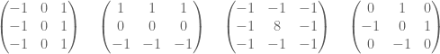
Note that, adding all the values of each matrix, one obtains zero. This is consistent with the third property required for our kernels: in the event of a locally flat area around a given pixel, convolution with any of these will offer a value of zero.

Read more…

Math Genealogy Project

I traced my mathematical lineage back into the XIV century at The Mathematics Genealogy Project. Imagine my surprise when I discovered that a big branch in the tree of my scientific ancestors is composed not by mathematicians, but by big names in the fields of Physics, Chemistry, Physiology and even Anatomy.

There is some “blue blood” in my family: Garrett Birkhoff, William Burnside (both algebrists). Archibald Hill, who shared the 1922 Nobel Prize in Medicine for his elucidation of the production of mechanical work in muscles. He is regarded, along with Hermann Helmholtz, as one of the founders of Biophysics.

Thomas Huxley (a.k.a. “Darwin’s Bulldog”, biologist and paleontologist) participated in that famous debate in 1860 with the Lord Bishop of Oxford, Samuel Wilberforce. This was a key moment in the wider acceptance of Charles Darwin’s Theory of Evolution.

There are some hard-core scientists in the XVIII century, like Joseph Barth and Georg Beer (the latter is notable for inventing the flap operation for cataracts, known today as Beer’s operation).

My namesake Franciscus Sylvius, another professor in Medicine, discovered the cleft in the brain now known as Sylvius’ fissure (circa 1637). One of his advisors, Jan Baptist van Helmont, is the founder of Pneumatic Chemistry and disciple of Paracelsus, the father of Toxicology (for some reason, the Mathematics Genealogy Project does not list any of these two in my lineage—I wonder why).

There are other big names among the branches of my scientific genealogy tree, but I will postpone this discovery towards the end of the post, for a nice punch-line.

Posters with your genealogy are available for purchase from the pages of the Mathematics Genealogy Project, but they are not very flexible neither in terms of layout nor design in general. A great option is, of course, doing it yourself. With the aid of python, GraphViz and a the sage library networkx, this becomes a straightforward task. Let me show you a naïve way to accomplish it:

Basic Statistics in sage

No need to spend big bucks in the purchase of expensive statistical software packages (SPSS or SAS): the R programming language will do it all for you, and of course sage has a neat way to interact with it. Let me prove you its capabilities with an example taken from one of the many textbooks used to teach the practice of basic statistics to researchers of Social Sciences (sorry, no names, unless you want to pay for the publicity!)

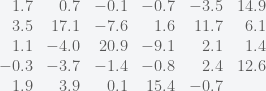
Estimating Mean Weight Change for Anorexic Girls

The example comes from an experimental study that compared various treatments for young girls suffering from anorexia, an eating disorder. For each girl, weight was measured before and after a fixed period of treatment. The variable of interest was the change in weight; that is, weight at the end of the study minus weight at the beginning of the study. The change in weight was positive if the girl gained weight, and negative if she lost weight. The treatments were designed to aid weight gain. The weight changes for the 29 girls undergoing the cognitive behavioral treatment were

Toying with basic fractals

I will skip all the mathematical theory behind Fractals (dimensions, measures, etc) to focus directly into the description and implementation of some of the most basic examples. In this post, I will cover the ideas behind three classical techniques:

• Iterated function systems
• Membership tests
• Lindenmayer systems

Wavelets in sage

There are no native wavelet packages in sage. But there is a great module in python that contains, among other things, forward and inverse discrete wavelet transforms (for one and two dimensions). It comes bundled with seventy-six wavelet filters, and allows support to build your own! The name is PyWavelets, written by Tariq Rashid, and can be retrieved from pypi.python.org/pypi/PyWavelets. In order to install it in sage, take the following steps:

Read more…

Edge detection: The Scale Space Theory

Consider an image as a bounded function with no smoothness or structure assumptions a priori. Most relevant information of a given image is contained in the contours of the mapped objects: Think for example of a bright object against a dark background—the area where these two meet presents a curve where the intensity varies strongly. This is what we refer to as an “edge.”

Initially, we may consider the process of detection of an edge by the simple computation of the gradient This gradient should have a large intensity and a direction which indicates the perpendicular to the curve. It therefore looks sound to simply compute the gradient of and choose the points where these values are large. This conclusion is a bit unrealistic for two reasons:

1. The points where the gradient is larger than a given threshold are open sets, and thus don’t have the structure of curves.
2. Large gradient may arise in certain locations of the image due to tiny oscillations or noise, but completely unrelated to the objects being mapped. As a matter of fact, there is no reason to assume the existence or computability of any gradient at all in a given digital image.

Read more…

Voronoi mosaics

While looking for ideas to implement voronoi in sage, I stumbled upon a beautiful paper written by a group of japanese computer graphic professionals from the universities of Hokkaido and Tokyo: A Method for Creating Mosaic Images Using Voronoi Diagrams. The first step of their algorithm is simple yet brilliant: Start with any given image, and superimpose an hexagonal tiling of the plane. By a clever approximation scheme, modify the tiling to become a voronoi diagram that adaptively minimizes some approximation error. As a consequence, the resulting voronoi diagram is somehow adapted to the desired contours of the original image.

(Fig. 1)	(Fig. 2)	(Fig. 3)	(Fig. 4)

In a second step, they manually adjust the Voronoi image interactively by moving, adding, or deleting sites. They also take the liberty of adding visual effects by hand: emphasizing the outlines and color variations in each Voronoi region, so they look like actual pieces of stained glass (Fig. 4).

Image Processing with numpy, scipy and matplotlibs in sage

In this post, I would like to show how to use  a few different features of numpy, scipy and matplotlibs to accomplish a few basic image processing tasks: some trivial image manipulation, segmentation, obtaining of structural information, etc.  An excellent way to show a good set of these techniques is by working through a complex project.  In this case, I have chosen the following:

Given a HAADF-STEM micrograph of a bronze-type Niobium Tungsten oxide (left), find a script that constructs a good approximation to its structural model (right).

Courtesy of ETH Zurich

For pedagogical purposes, I took the following approach to solving this problem:

1. Segmentation of the atoms by thresholding and morphological operations.
2. Connected component labeling to extract each single atom for posterior examination.
3. Computation of the centers of mass of each label identified as an atom. This presents us with a lattice of points in the plane that shows a first insight in the structural model of the oxide.
4. Computation of Delaunay triangulation and Voronoi diagram of the previous lattice of points. The combination of information from these two graphs will lead us to a decent (approximation to the actual) structural model of our sample.

Let us proceed in this direction: