Basic Statistics in sage

No need to spend big bucks in the purchase of expensive statistical software packages (SPSS or SAS): the R programming language will do it all for you, and of course sage has a neat way to interact with it. Let me prove you its capabilities with an example taken from one of the many textbooks used to teach the practice of basic statistics to researchers of Social Sciences (sorry, no names, unless you want to pay for the publicity!)

Estimating Mean Weight Change for Anorexic Girls

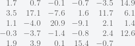
The example comes from an experimental study that compared various treatments for young girls suffering from anorexia, an eating disorder. For each girl, weight was measured before and after a fixed period of treatment. The variable of interest was the change in weight; that is, weight at the end of the study minus weight at the beginning of the study. The change in weight was positive if the girl gained weight, and negative if she lost weight. The treatments were designed to aid weight gain. The weight changes for the 29 girls undergoing the cognitive behavioral treatment were

Let us examine the data with the statistical tools that R offers us. We start by invoking this programming language in sage, loading the data, and issuing basic commands to explore its properties:

sage: %r

–> Switching to R Interpreter <–

”
r: A <- c(1.7,0.7,-0.1,-0.7,-3.5,14.9,3.5,17.1,-7.6,
1.6,11.7,6.1,1.1,-4.0,20.9,-9.1,2.1,1.4,
-0.3,-3.7,-1.4,-0.8,2.4,12.6,1.9,3.9,0.1,
15.4,-0.7)

r: summary(A)
Min. 1st Qu. Median Mean 3rd Qu. Max.
-9.100 -0.700 1.400 3.007 3.900 20.900
r: stem(A)

The decimal point is 1 digit(s) to the right of the |

-0 | 98
-0 | 444111100
0 | 01112222244
0 | 6
1 | 23
1 | 557
2 | 1

r: quartz()
r: hist(A)
r: boxplot(A)
r: dev.off()

Note the command quartz: this is to communicate with Mac OS X our wish to plot data to a window. There are similar commands to plot in Windows [windows()], in X11 [X11()], or even to save to file [png(), jpeg(), bmp(), tiff(), postcript(), …]. Make sure to read the help on their usage.

Let us try now a more complex task: Confidence interval for population mean. Although the histogram does not suggest a normal population distribution, we are confident that this method will give us a trustworthy result—using the t distribution for computation of confident intervals is robust, especially so when the size of the sample is larger than fifteen:

r: t.test(A)

One Sample t-test

data: A
t = 2.2156, df = 28, p-value = 0.03502
alternative hypothesis: true mean is not equal to 0
95 percent confidence interval:
0.2268902 5.7869029
sample estimates:
mean of x
3.006897

Note the information offered by the output: with 95% confidence, we infer that the interval contains the population mean weight change. How was this interval calculated? Since 29 girls received the treatment, there are 28 degrees of freedom. The mean weight change was and Can you infer at this point the values of the standard deviation and estimated standard error?

To be safer in estimating the population mean weight change, we could use instead a 99% confidence interval.

r: t.test(A,conf.level=0.99)

One Sample t-test

data: A
t = 2.2156, df = 28, p-value = 0.03502
alternative hypothesis: true mean is not equal to 0
99 percent confidence interval:
-0.7432794 6.7570725
sample estimates:
mean of x
3.006897

Note that at this confidence level, the interval contains zero. This tells us that it is plausible (at this level) that the therapy may not result in any change in the mean weight. Interesting, right?

Let us go a little further in this direction: Let denote the population mean change in weight for this cognitive bahavioral treatment. If the treatment has beneficial efects as expected, then must be positive. To test for no treatment effect vs. positive mean change, we test against Note that this is a one-sided alternative hypothesis, so let us modify our call of the t.test in R accordingly:

r: t.test(A,alternative=“greater”,conf.level=0.95)

One Sample t-test

data: A
t = 2.2156, df = 28, p-value = 0.01751
alternative hypothesis: true mean is greater than 0
95 percent confidence interval:
0.6981979 Inf
sample estimates:
mean of x
3.006897

It seems that the treatment has an effect!