Jotto (5-letter Mastermind) in the NAO robot

I would like to show how to code the NAO robot to beat us at Jotto (5-letter Mastermind) with python in Choregraphe. I will employ a brute force technique that does not require any knowledge of the English language, the frequency of its letters, or smart combinations of vowels and consonants to try to minimize the number of attempts. It goes like this:

1. Gather all 5-letter words with no repeated letters in a list.
2. Choose a random word from that list—your guess—, and ask it to be scored ala Mastermind.
3. Filter through the list all words that share the same score with your guess; discard the rest.
4. Go back to step 2 and repeat until the target word is found.

Coding this strategy in python requires only four variables:

• whole_dict: the list with all the words
• step = [x for x in whole_dict]: A copy of whole_dict, which is going to be shortened on each step (hence the name). Note that stating step = whole_dict will change the contents of whole_dict when we change the contents of step — not a good idea.
• guess = random.choice(step): A random choice from the list step.
• score: A string containing the two digits we obtain after scoring the guess. The first digit indicates the number of correct letters in the same position as the target word; the second digit indicates the number of correct letters in the wrong position.
• attempts: optional. The number of attempts at guessing words. For quality control purposes.

At this point, I urge the reader to stop reading the post and try to implement this strategy as a simple script. When done, come back to see how it can be coded in the NAO robot.

Robot stories

Every summer before school was over, I was assigned a list of books to read. Mostly nonfiction and historical fiction, but in fourth grade there that was that first science fiction book. I often remember how that book made me feel, and marvel at the impact that it had in my life. I had read some science fiction before—Well’s Time Traveller and War of the Worlds—but this was different. This was a book with witty and thought-provoking short stories by Isaac Asimov. Each of them delivered drama, comedy, mystery and a surprise ending in about ten pages. And they had robots. And those robots had personalities, in spite of their very simple programming: The Three Laws of Robotics.

1. A robot may not injure a human being or, through inaction, allow a human being to come to harm.
2. A robot must obey the orders given to it by human beings, except where such orders would conflict with the First Law.
3. A robot must protect its own existence as long as such protection does not conflict with the First or Second Law.

Back in the 1980s, robotics—understood as autonomous mechanical thinking—was no more than a dream. A wonderful dream that fueled many children’s imaginations and probably shaped the career choices of some. I know in my case it did.

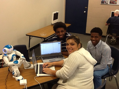
Fast forward some thirty-odd years, when I met Astro: one of three research robots manufactured by the French company Aldebaran. This NAO robot found its way into the computer science classroom of Tom Simpson in Heathwood Hall Episcopal School, and quickly learned to navigate mazes, recognize some student’s faces and names, and even dance the Macarena! It did so with effortless coding: a basic command of the computer language python, and some idea of object oriented programming.

I could not let this opportunity pass. I created a small undergraduate team with Danielle Talley from USC (a brilliant sophomore in computer engineering, with a minor in music), and two math majors from Morris College: my Geometry expert Fabian Maple, and a McGyver-style problem solver, Wesley Alexander. Wesley and Fabian are supported by a Department of Energy-Environmental Management grant to Morris College, which funds their summer research experience at USC. Danielle is funded by the National Science Foundation through the Louis Stokes South Carolina-Alliance for Minority Participation (LS-SCAMP).

They spent the best of their first week on this project completing a basic programming course online. At the same time, the four of us reviewed some of the mathematical tools needed to teach Astro new tricks: basic algebra and trigonometry, basic geometry, and basic calculus and statistics. The emphasis—I need to point out in case you missed it—is in the word basic.

Talk the talk

The psychologist seated herself and watched Herbie narrowly as he took a chair at the other side of the table and went through the three books systematically.

At the end of half an hour, he put them down, “Of course, I know why you brought these.”

The corner of Dr. Calvin’s lip twitched, “I was afraid you would. It’s difficult to work with you, Herbie. You’re always a step ahead of me.”

“It’s the same with these books, you know, as with the others. They just don’t interest me. There’s nothing to your textbooks. Your science is just a mass of collected data plastered together by makeshift theory — and all so incredibly simple, that it’s scarcely worth bothering about.”

“It’s your fiction that interests me. Your studies of the interplay of human motives and emotions” – his mighty hand gestured vaguely as he sought the proper words.

Liar!
— Isaac Asimov

Astro can understand what I say, and maintain conversations with me. He has four microphones for voice recognition and sound localization, and two speakers for text-to-speech synthesis. But he sometimes gets confused: I say “acute”, and he understands “abide,” for example. This might sound frustrating by all standards. But mathematicians can’t be judged by any reasonable standard. Far from seeing this as a shortcoming, my team used as motivation the mechanics behind his speech recognition functionality, and they wrote some code to turn him into an expert Mastermind player.

Wait, what? How are these two things possibly connected?

Since Astro’s hearing is far from perfect, when he hears a word which is not clear, he gathers a short list of possible candidates. He then chooses the most likely guess based upon different considerations—using clues from context, for example. Based on similar strategies, he can be taught to be a perfect player of 5-letter-word Mastermind: Pick any five-letter word in the English language. Any word, provided it has no repeated letters. Astro chooses one random word as his first guess, and requests a score like in Mastermind.

To illustrate this process, I will show you how the game went when I chose Fabian’s favorite word: “acute.”

Astro: Is it firth?
Me   : NO
Astro: How many letters of my guess are in your word, in the right position?
       How many letters of my guess are in your word, in the wrong position?
Me   : 1, 0
Astro: Is it foams?
Me   : NO
Astro: How many letters of my guess are in your word, in the right position?
       How many letters of my guess are in your word, in the wrong position?
Me   : 0, 1
Astro: Is it junta?
Me   : NO
Astro: How many letters of my guess are in your word, in the right position?
       How many letters of my guess are in your word, in the wrong position?
Me   : 1, 2
Astro: Is it acute?
Me   : YES
Astro: Wonderful, I found it in 4 attempts!

I don’t want to get too technical here, but will mention some of the ideas. The main algorithm is based on techniques of numerical root finding and solving nonlinear equations — nothing complex: high-school level bracketing by bisection, or Newton’s method. To design better winning strategies, my team exploits the benefits of randomness. The analysis of this part is done with basic probability and statistics.

Walk the walk

Donovan’s pencil pointed nervously. “The red cross is the selenium pool. You marked it yourself.”

“Which one is it?” interrupted Powell. “There were three that MacDougal located for us before he left.”

“I sent Speedy to the nearest, naturally; seventeen miles away. But what difference does that make?” There was tension in his voice. “There are penciled dots that mark Speedy’s position.”

And for the first time Powell’s artificial aplomb was shaken and his hands shot forward for the man.

“Are you serious? This is impossible.”

“There it is,” growled Donovan.

The little dots that marked the position formed a rough circle about the red cross of the selenium pool. And Powell’s fingers went to his brown mustache, the unfailing signal of anxiety.

Donovan added: “In the two hours I checked on him, he circled that damned pool four times. It seems likely to me that he’ll keep that up forever. Do you realize the position we’re in?”

Runaround
— Isaac Asimov

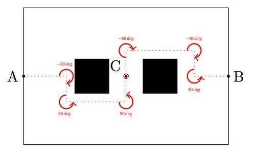
Astro moves around too. It does so thanks to a sophisticated system combining one accelerometer, one gyrometer and four ultrasonic sensors that provide him with stability and positioning within space. He also enjoys eight force-sensing resistors and two bumpers. And that is only for his legs! He can move his arms, bend his elbows, open and close his hands, or move his torso and neck (up to 25 degrees of freedom for the combination of all possible joints). Out of the box, and without much effort, he can be coded to walk around, although in a mechanical way: He moves forward a few feet, stops, rotates in place or steps to a side, etc. A very naïve way to go from A to B retrieving an object at C, could be easily coded in this fashion as the diagram shows:

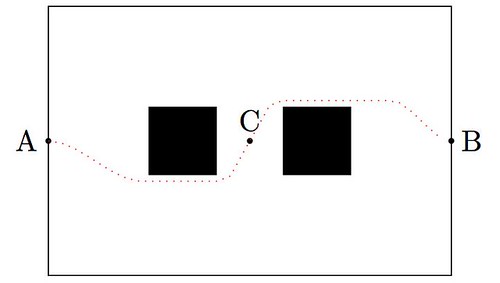
Fabian and Wesley devised a different way to code Astro taking full advantage of his inertial measurement unit. This will allow him to move around smoothly, almost like a human would. The key to their success? Polynomial interpolation and plane geometry. For advanced solutions, they need to learn about splines, curvature, and optimization. Nothing they can’t handle.

Sing me a song

He said he could manage three hours and Mortenson said that would be perfect when I gave him the news. We picked a night when she was going to be singing Bach or Handel or one of those old piano-bangers, and was going to have a long and impressive solo.

Mortenson went to the church that night and, of course, I went too. I felt responsible for what was going to happen and I thought I had better oversee the situation.

Mortenson said, gloomily, “I attended the rehearsals. She was just singing the same way she always did; you know, as though she had a tail and someone was stepping on it.”

One Night of Song
— Isaac Asimov

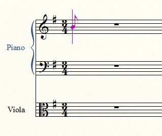
Astro has excellent eyesight and understanding of the world around him. He is equipped with two HD cameras, and a bunch of computer vision algorithms, including facial and shape recognition. Danielle’s dream is to have him read from a music sheet and sing or play the song in a toy piano. She is very close to completing this project: Astro is able now to identify partitures, and extract from them the location of the pentagrams. Danielle is currently working on identifying the notes and the clefs. This is one of her test images, and the result of one of her early experiments:

Most of the techniques Danielle is using are accessible to any student with a decent command of vector calculus, and enough scientific maturity. The extraction of pentagrams and the different notes on them, for example, is performed with the Hough transform. This is a fancy term for an algorithm that basically searches for straight lines and circles by solving an optimization problem in two or three variables.

The only thing left is an actual performance. Danielle will be leading Fabian and Wes, and with the assistance of Mr. Simpson’s awesome students Erica and Robert, Astro will hopefully learn to physically approach the piano, choose the right keys, and play them in the correct order and speed. Talent show, anyone?

Book presentation at the USC Python Users Group

More on Lindenmayer Systems

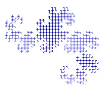
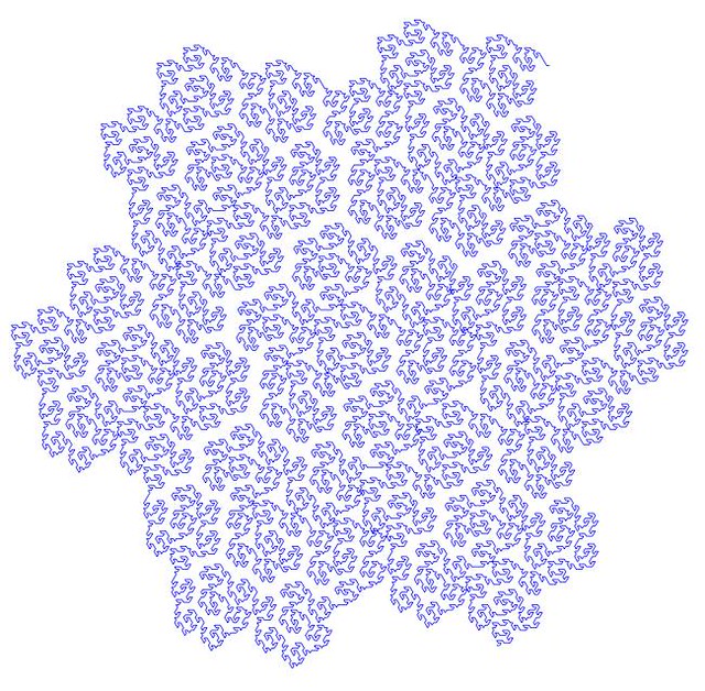
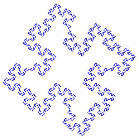
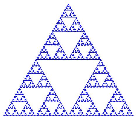
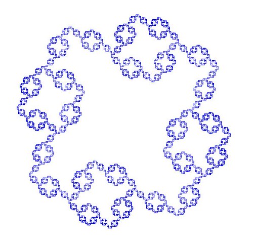
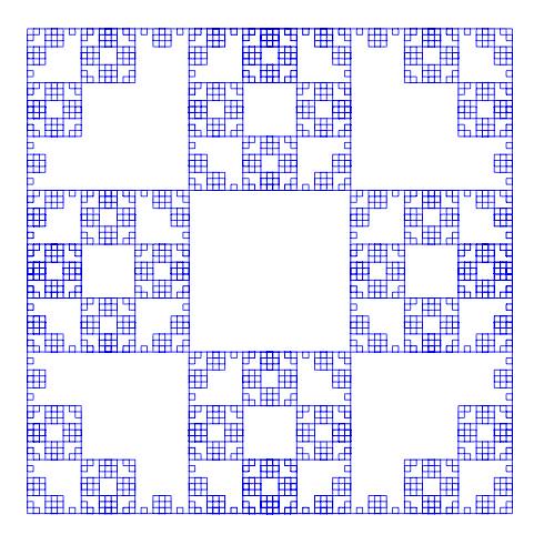
We briefly explored Lindenmayer systems (or L-systems) in an old post: Toying with Basic Fractals. We quickly reviewed this method for creation of an approximation to fractals, and displayed an example (the Koch snowflake) based on tikz libraries.

I would like to show a few more examples of beautiful curves generated with this technique, together with their generating axiom, rules and parameters. Feel free to click on each of the images below to download a larger version.

Note that any coding language with plotting capabilities should be able to tackle this project. I used once again tikz for , but this time with the tikzlibrary lindenmayersystems.

name : Dragon Curve axiom : X order : 11 step : 5pt angle : 90 rules : X -> X+YF+ Y -> -FX-Y	name : Gosper Space-filling Curve axiom : XF order : 5 step : 2pt angle : 60 rules : XF -> XF+YF++YF-XF--XFXF-YF+ YF -> -XF+YFYF++YF+XF--XF-YF
name : Quadric Koch Island axiom : F+F+F+F order : 4 step : 1pt angle : 90 rules : F -> F+F-F-FF+F+F-F	name : Sierpinski Arrowhead axiom : F order : 8 step : 3.5pt angle : 60 rules : G -> F+G+F F -> G-F-G
name : ? axiom : F+F+F+F order : 4 step : 2pt angle : 90 rules : F -> FF+F+F+F+F+F-F	name : ? axiom : F+F+F+F order : 4 step : 3pt angle : 90 rules : F -> FF+F+F+F+FF

Would you like to experiment a little with axioms, rules and parameters, and obtain some new pleasant curves with this method? If the mathematical properties of the fractal that they approximate are interesting enough, I bet you could attach your name to them. Like the astronomer that finds through her telescope a new object in the sky, or the zoologist that discover a new species of spider in the forest.

Sympy should suffice

I have just received a copy of Instant SymPy Starter, by Ronan Lamy—a no-nonsense guide to the main properties of SymPy, the Python library for symbolic mathematics. This short monograph packs everything you should need, with neat examples included, in about 50 pages. Well-worth its money.

To celebrate, I would like to pose a few coding challenges on the use of this library, based on a fun geometric puzzle from cut-the-knot: Rhombus in Circles

Segments and are equal. Lines and intersect at Form four circumcircles: Prove that the circumcenters form a rhombus, with

Note that if this construction works, it must do so independently of translations, rotations and dilations. We may then assume that is the origin, that the segments have length one, and that for some parameters it is We let SymPy take care of the computation of circumcenters:

import sympy
from sympy import *

# Point definitions
M=Point(0,0)
A=Point(2,0)
B=Point(1,0)
a,theta=symbols('a,theta',real=True,positive=True)
C=Point((a+1)*cos(theta),(a+1)*sin(theta))
D=Point(a*cos(theta),a*sin(theta))

#Circumcenters
E=Triangle(A,C,M).circumcenter
F=Triangle(A,D,M).circumcenter
G=Triangle(B,D,M).circumcenter
H=Triangle(B,C,M).circumcenter

Finding that the alternate angles are equal in the quadrilateral is pretty straightforward:

In [11]: P=Polygon(E,F,G,H)

In [12]: P.angles[E]==P.angles[G]
Out[12]: True

In [13]: P.angles[F]==P.angles[H]
Out[13]: True

To prove it a rhombus, the two sides that coincide on each angle must be equal. This presents us with the first challenge: Note for example that if we naively ask SymPy whether the triangle is equilateral, we get a False statement:

In [14]: Triangle(E,F,G).is_equilateral()
Out[14]: False

In [15]: F.distance(E)
Out[15]: Abs((a/2 - cos(theta))/sin(theta) - (a - 2*cos(theta) + 1)/(2*sin(theta)))

In [16]: F.distance(G)
Out[16]: sqrt(((a/2 - cos(theta))/sin(theta) - (a - cos(theta))/(2*sin(theta)))**2 + 1/4)

Part of the reason is that we have not indicated anywhere that the parameter theta is to be strictly bounded above by (we did indicate that it must be strictly positive). The other reason is that SymPy does not handle identities well, unless the expressions to be evaluated are perfectly simplified. For example, if we trust the routines of simplification of trigonometric expressions alone, we will not be able to resolve this problem with this technique:

In [17]: trigsimp(F.distance(E)-F.distance(G),deep=True)==0
Out[17]: False

Finding that with SymPy is not that easy either. This is the second challenge.

How would the reader resolve this situation?

Instant SymPy Starter

Naïve Bayes

There is nothing naïve about Naïve Bayes—a very basic, but extremely efficient data mining method to take decisions when a vast amount of data is available. The name comes from the fact that this is the simplest application to this problem, upon (the naïve) assumption of independence of the events. It is based on Bayes’ rule of conditional probability: If you have a hypothesis and evidence that bears on that hypothesis, then

where as usual, denotes the probability of the event and denotes the probability of the event conditional to another event

I would like to show an example of this technique, of course, with yet another decision-making algorithm oriented to guess my reaction to a movie I have not seen before. From the data obtained in a previous post, I create a simpler table with only those movies that have been scored more than 28 times (by a pool of 87 of the most popular critics featured in www.metacritics.com) [I posted the script to create that table at the end of the post]

Let’s test it:

>>> table=prepTable(scoredMovies,28)
>>> len(table)

49
>>> [entry[0] for entry in table]

[‘rabbit-hole’, ‘carnage-2011’, ‘star-wars-episode-iii—revenge-of-the-sith’,
‘shame’, ‘brokeback-mountain’, ‘drive’, ‘sideways’, ‘salt’,
‘million-dollar-baby’, ‘a-separation’, ‘dark-shadows’,
‘the-lord-of-the-rings-the-return-of-the-king’, ‘true-grit’, ‘inception’,
‘hereafter’, ‘master-and-commander-the-far-side-of-the-world’, ‘batman-begins’,
‘harry-potter-and-the-deathly-hallows-part-2’, ‘the-artist’, ‘the-fighter’,
‘larry-crowne’, ‘the-hunger-games’, ‘the-descendants’, ‘midnight-in-paris’,
‘moneyball’, ‘8-mile’, ‘the-departed’, ‘war-horse’,
‘the-lord-of-the-rings-the-fellowship-of-the-ring’, ‘j-edgar’,
‘the-kings-speech’, ‘super-8’, ‘robin-hood’, ‘american-splendor’, ‘hugo’,
‘eternal-sunshine-of-the-spotless-mind’, ‘the-lovely-bones’, ‘the-tree-of-life’,
‘the-pianist’, ‘the-ides-of-march’, ‘the-quiet-american’, ‘alexander’,
‘lost-in-translation’, ‘seabiscuit’, ‘catch-me-if-you-can’, ‘the-avengers-2012’,
‘the-social-network’, ‘closer’, ‘the-girl-with-the-dragon-tattoo-2011’]
>>> table[0]

[‘rabbit-hole’, ”, ‘B+’, ‘B’, ”, ‘C’, ‘C+’, ”, ‘F’, ‘B+’, ‘F’, ‘C’, ‘F’, ‘D’,
”, ”, ‘A’, ”, ”, ”, ”, ‘B+’, ‘C+’, ”, ”, ”, ”, ”, ”, ‘C+’, ”, ”,
”, ”, ”, ”, ‘A’, ”, ”, ”, ”, ”, ‘A’, ”, ”, ‘B+’, ‘B+’, ‘B’, ”, ”,
”, ‘D’, ‘B+’, ”, ”, ‘C+’, ”, ”, ”, ”, ”, ”, ‘B+’, ”, ”, ”, ”, ”,
”, ‘A’, ”, ”, ”, ”, ”, ”, ”, ‘D’, ”, ”,’C+’, ‘A’, ”, ”, ”, ‘C+’, ”]

Math still not the answer

I wrote a quick (but not very elegant) python script to retrieve locally enough data from www.metacritic.com for pattern recognition purposes. The main goal is to help me decide how much I will enjoy a movie, before watching it. I included the script at the end of the post, in case you want to try it yourself (and maybe improve it too!). It takes a while to complete, although it is quite entertaining to see its progress on screen. At the end, it provides with two lists of the same length: critics—a list of str containing the names of the critics; and scoredMovies—a list of dict containing, at index k, the evaluation of all the movies scored by the critic at index k in the previous list.

For example:

>>> critics[43]

‘James White’
>>> scoredMovies[43]

{‘hall-pass’: 60, ‘the-karate-kid’: 60, ‘the-losers’: 60,
‘the-avengers-2012’: 80, ‘the-other-guys’: 60, ‘shrek-forever-after’: 80,
‘the-lincoln-lawyer’: 80, ‘the-company-men’: 60, ‘jonah-hex’: 40,
‘arthur’: 60, ‘vampires-suck’: 20, ‘american-reunion’: 40,
‘footloose’: 60, ‘real-steel’: 60}

The number of scored films by critic varies: there are individuals that gave their opinion on a few dozen movies, and others that took the trouble to evaluate up to four thousand flicks! Note also that the names of the movies correspond with their web pages in www.metacritic.com. For example, to see what critics have to say about the “Karate Kid” and other relevant information online, point your browser to www.metacritic.com/movie/the-karate-kid. It also comes in very handy if there are several versions of a single title: Which “Karate Kid” does this score refer to, the one in the eighties, or Jackie Chan’s?

Feel free to download a copy of the resulting data [here] (note it is a large file: 1.6MB).

But the fact that we have that data stored locally allows us to gather that information with simple python commands, and perform many complex operations on it.

Edge detection: The Convolution Approach

Today I would like to show a very basic technique of detection based on simple convolution of an image with small kernels (masks). The purpose of these kernels is to enhance certain properties of the image at each pixel. What properties? Those that define what means to be an edge, in a differential calculus way—exactly as it was defined in the description of the Canny edge detector. The big idea is to assign to each pixel a numerical value that expresses its strength as an edge: positive if we suspect that such structure is present at that location, negative if not, and zero if the image is locally flat around that point. Masks can be designed so that they mimic the effect of differential operators, but these can be terribly complicated and give rise to large matrices.

The first approaches were performed with simple kernels. For example, Faler came up with the following four simple masks that emulate differentiation:

Note that, adding all the values of each matrix, one obtains zero. This is consistent with the third property required for our kernels: in the event of a locally flat area around a given pixel, convolution with any of these will offer a value of zero.

Read more…

Math Genealogy Project

I traced my mathematical lineage back into the XIV century at The Mathematics Genealogy Project. Imagine my surprise when I discovered that a big branch in the tree of my scientific ancestors is composed not by mathematicians, but by big names in the fields of Physics, Chemistry, Physiology and even Anatomy.

There is some “blue blood” in my family: Garrett Birkhoff, William Burnside (both algebrists). Archibald Hill, who shared the 1922 Nobel Prize in Medicine for his elucidation of the production of mechanical work in muscles. He is regarded, along with Hermann Helmholtz, as one of the founders of Biophysics.

Thomas Huxley (a.k.a. “Darwin’s Bulldog”, biologist and paleontologist) participated in that famous debate in 1860 with the Lord Bishop of Oxford, Samuel Wilberforce. This was a key moment in the wider acceptance of Charles Darwin’s Theory of Evolution.

There are some hard-core scientists in the XVIII century, like Joseph Barth and Georg Beer (the latter is notable for inventing the flap operation for cataracts, known today as Beer’s operation).

My namesake Franciscus Sylvius, another professor in Medicine, discovered the cleft in the brain now known as Sylvius’ fissure (circa 1637). One of his advisors, Jan Baptist van Helmont, is the founder of Pneumatic Chemistry and disciple of Paracelsus, the father of Toxicology (for some reason, the Mathematics Genealogy Project does not list any of these two in my lineage—I wonder why).

There are other big names among the branches of my scientific genealogy tree, but I will postpone this discovery towards the end of the post, for a nice punch-line.

Posters with your genealogy are available for purchase from the pages of the Mathematics Genealogy Project, but they are not very flexible neither in terms of layout nor design in general. A great option is, of course, doing it yourself. With the aid of python, GraphViz and a the sage library networkx, this becomes a straightforward task. Let me show you a naïve way to accomplish it:

Wavelets in sage

There are no native wavelet packages in sage. But there is a great module in python that contains, among other things, forward and inverse discrete wavelet transforms (for one and two dimensions). It comes bundled with seventy-six wavelet filters, and allows support to build your own! The name is PyWavelets, written by Tariq Rashid, and can be retrieved from pypi.python.org/pypi/PyWavelets. In order to install it in sage, take the following steps:

Read more…