Computational Geometry in Python

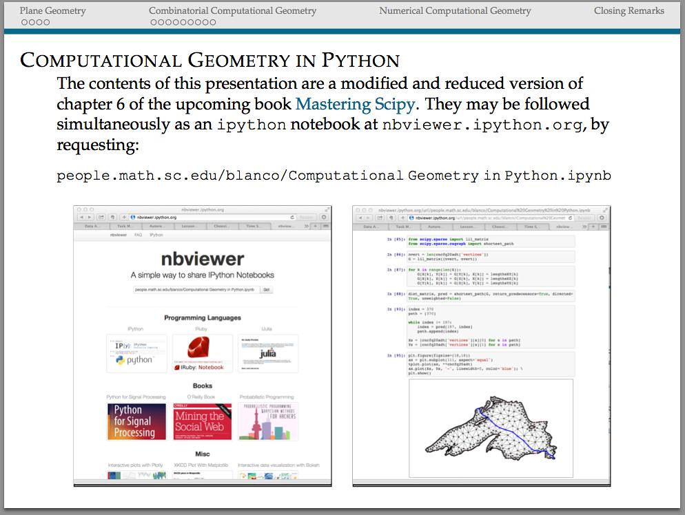
To illustrate a few advantages of the scipy stack in one of my upcoming talks, I have placed an ipython notebook with (a reduced version of) the current draft of Chapter 6 (Computational Geometry) of my upcoming book: Mastering SciPy.

The raw ipynb can be downloaded from my github repository [blancosilva/Mastering-Scipy/], or viewed directly from the nbviewer at [this other link]

I also made a selection with some fun examples for the talk. You can download the presentation by clicking in the image above.

Enjoy!

Robot stories

Every summer before school was over, I was assigned a list of books to read. Mostly nonfiction and historical fiction, but in fourth grade there that was that first science fiction book. I often remember how that book made me feel, and marvel at the impact that it had in my life. I had read some science fiction before—Well’s Time Traveller and War of the Worlds—but this was different. This was a book with witty and thought-provoking short stories by Isaac Asimov. Each of them delivered drama, comedy, mystery and a surprise ending in about ten pages. And they had robots. And those robots had personalities, in spite of their very simple programming: The Three Laws of Robotics.

1. A robot may not injure a human being or, through inaction, allow a human being to come to harm.
2. A robot must obey the orders given to it by human beings, except where such orders would conflict with the First Law.
3. A robot must protect its own existence as long as such protection does not conflict with the First or Second Law.

Back in the 1980s, robotics—understood as autonomous mechanical thinking—was no more than a dream. A wonderful dream that fueled many children’s imaginations and probably shaped the career choices of some. I know in my case it did.

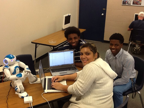
Fast forward some thirty-odd years, when I met Astro: one of three research robots manufactured by the French company Aldebaran. This NAO robot found its way into the computer science classroom of Tom Simpson in Heathwood Hall Episcopal School, and quickly learned to navigate mazes, recognize some student’s faces and names, and even dance the Macarena! It did so with effortless coding: a basic command of the computer language python, and some idea of object oriented programming.

I could not let this opportunity pass. I created a small undergraduate team with Danielle Talley from USC (a brilliant sophomore in computer engineering, with a minor in music), and two math majors from Morris College: my Geometry expert Fabian Maple, and a McGyver-style problem solver, Wesley Alexander. Wesley and Fabian are supported by a Department of Energy-Environmental Management grant to Morris College, which funds their summer research experience at USC. Danielle is funded by the National Science Foundation through the Louis Stokes South Carolina-Alliance for Minority Participation (LS-SCAMP).

They spent the best of their first week on this project completing a basic programming course online. At the same time, the four of us reviewed some of the mathematical tools needed to teach Astro new tricks: basic algebra and trigonometry, basic geometry, and basic calculus and statistics. The emphasis—I need to point out in case you missed it—is in the word basic.

Talk the talk

The psychologist seated herself and watched Herbie narrowly as he took a chair at the other side of the table and went through the three books systematically.

At the end of half an hour, he put them down, “Of course, I know why you brought these.”

The corner of Dr. Calvin’s lip twitched, “I was afraid you would. It’s difficult to work with you, Herbie. You’re always a step ahead of me.”

“It’s the same with these books, you know, as with the others. They just don’t interest me. There’s nothing to your textbooks. Your science is just a mass of collected data plastered together by makeshift theory — and all so incredibly simple, that it’s scarcely worth bothering about.”

“It’s your fiction that interests me. Your studies of the interplay of human motives and emotions” – his mighty hand gestured vaguely as he sought the proper words.

Liar!
— Isaac Asimov

Astro can understand what I say, and maintain conversations with me. He has four microphones for voice recognition and sound localization, and two speakers for text-to-speech synthesis. But he sometimes gets confused: I say “acute”, and he understands “abide,” for example. This might sound frustrating by all standards. But mathematicians can’t be judged by any reasonable standard. Far from seeing this as a shortcoming, my team used as motivation the mechanics behind his speech recognition functionality, and they wrote some code to turn him into an expert Mastermind player.

Wait, what? How are these two things possibly connected?

Since Astro’s hearing is far from perfect, when he hears a word which is not clear, he gathers a short list of possible candidates. He then chooses the most likely guess based upon different considerations—using clues from context, for example. Based on similar strategies, he can be taught to be a perfect player of 5-letter-word Mastermind: Pick any five-letter word in the English language. Any word, provided it has no repeated letters. Astro chooses one random word as his first guess, and requests a score like in Mastermind.

To illustrate this process, I will show you how the game went when I chose Fabian’s favorite word: “acute.”

Astro: Is it firth?
Me   : NO
Astro: How many letters of my guess are in your word, in the right position?
       How many letters of my guess are in your word, in the wrong position?
Me   : 1, 0
Astro: Is it foams?
Me   : NO
Astro: How many letters of my guess are in your word, in the right position?
       How many letters of my guess are in your word, in the wrong position?
Me   : 0, 1
Astro: Is it junta?
Me   : NO
Astro: How many letters of my guess are in your word, in the right position?
       How many letters of my guess are in your word, in the wrong position?
Me   : 1, 2
Astro: Is it acute?
Me   : YES
Astro: Wonderful, I found it in 4 attempts!

I don’t want to get too technical here, but will mention some of the ideas. The main algorithm is based on techniques of numerical root finding and solving nonlinear equations — nothing complex: high-school level bracketing by bisection, or Newton’s method. To design better winning strategies, my team exploits the benefits of randomness. The analysis of this part is done with basic probability and statistics.

Walk the walk

Donovan’s pencil pointed nervously. “The red cross is the selenium pool. You marked it yourself.”

“Which one is it?” interrupted Powell. “There were three that MacDougal located for us before he left.”

“I sent Speedy to the nearest, naturally; seventeen miles away. But what difference does that make?” There was tension in his voice. “There are penciled dots that mark Speedy’s position.”

And for the first time Powell’s artificial aplomb was shaken and his hands shot forward for the man.

“Are you serious? This is impossible.”

“There it is,” growled Donovan.

The little dots that marked the position formed a rough circle about the red cross of the selenium pool. And Powell’s fingers went to his brown mustache, the unfailing signal of anxiety.

Donovan added: “In the two hours I checked on him, he circled that damned pool four times. It seems likely to me that he’ll keep that up forever. Do you realize the position we’re in?”

Runaround
— Isaac Asimov

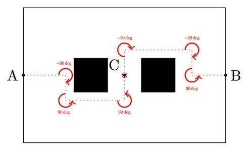
Astro moves around too. It does so thanks to a sophisticated system combining one accelerometer, one gyrometer and four ultrasonic sensors that provide him with stability and positioning within space. He also enjoys eight force-sensing resistors and two bumpers. And that is only for his legs! He can move his arms, bend his elbows, open and close his hands, or move his torso and neck (up to 25 degrees of freedom for the combination of all possible joints). Out of the box, and without much effort, he can be coded to walk around, although in a mechanical way: He moves forward a few feet, stops, rotates in place or steps to a side, etc. A very naïve way to go from A to B retrieving an object at C, could be easily coded in this fashion as the diagram shows:

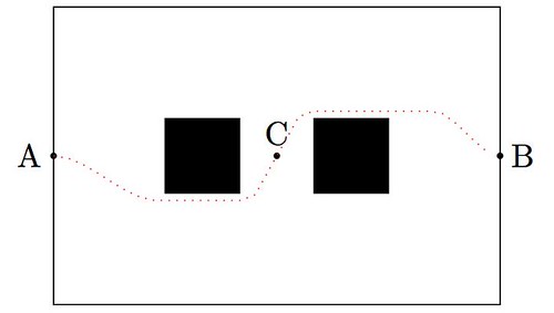
Fabian and Wesley devised a different way to code Astro taking full advantage of his inertial measurement unit. This will allow him to move around smoothly, almost like a human would. The key to their success? Polynomial interpolation and plane geometry. For advanced solutions, they need to learn about splines, curvature, and optimization. Nothing they can’t handle.

Sing me a song

He said he could manage three hours and Mortenson said that would be perfect when I gave him the news. We picked a night when she was going to be singing Bach or Handel or one of those old piano-bangers, and was going to have a long and impressive solo.

Mortenson went to the church that night and, of course, I went too. I felt responsible for what was going to happen and I thought I had better oversee the situation.

Mortenson said, gloomily, “I attended the rehearsals. She was just singing the same way she always did; you know, as though she had a tail and someone was stepping on it.”

One Night of Song
— Isaac Asimov

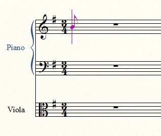
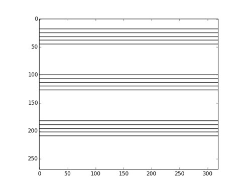
Astro has excellent eyesight and understanding of the world around him. He is equipped with two HD cameras, and a bunch of computer vision algorithms, including facial and shape recognition. Danielle’s dream is to have him read from a music sheet and sing or play the song in a toy piano. She is very close to completing this project: Astro is able now to identify partitures, and extract from them the location of the pentagrams. Danielle is currently working on identifying the notes and the clefs. This is one of her test images, and the result of one of her early experiments:

Most of the techniques Danielle is using are accessible to any student with a decent command of vector calculus, and enough scientific maturity. The extraction of pentagrams and the different notes on them, for example, is performed with the Hough transform. This is a fancy term for an algorithm that basically searches for straight lines and circles by solving an optimization problem in two or three variables.

The only thing left is an actual performance. Danielle will be leading Fabian and Wes, and with the assistance of Mr. Simpson’s awesome students Erica and Robert, Astro will hopefully learn to physically approach the piano, choose the right keys, and play them in the correct order and speed. Talent show, anyone?

Book presentation at the USC Python Users Group

Areas of Mathematics

For one of my upcoming talks I am trying to include an exhaustive mindmap showing the different areas of Mathematics, and somehow, how they relate to each other. Most of the information I am using has been processed from years of exposure in the field, and a bit of help from Wikipedia.

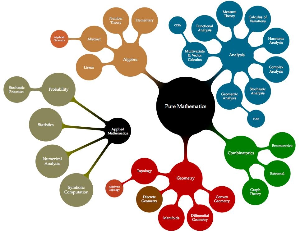
But I am not entirely happy with what I see: my lack of training in the area of Combinatorics results in a rather dry treatment of that part of the mindmap, for example. I am afraid that the same could be told about other parts of the diagram. Any help from the reader to clarify and polish this information will be very much appreciated.

And as a bonus, I included a script to generate the diagram with the aid of the tikz libraries.

\tikzstyle{level 2 concept}+=[sibling angle=40]
\begin{tikzpicture}[scale=0.49, transform shape]
  \path[mindmap,concept color=black,text=white]
    node[concept] {Pure Mathematics} [clockwise from=45]
      child[concept color=DeepSkyBlue4]{
        node[concept] {Analysis} [clockwise from=180]
          child { 
            node[concept] {Multivariate \& Vector Calculus}
              [clockwise from=120]
              child {node[concept] {ODEs}}}
              child { node[concept] {Functional Analysis}}
              child { node[concept] {Measure Theory}}
              child { node[concept] {Calculus of Variations}}
              child { node[concept] {Harmonic Analysis}}
              child { node[concept] {Complex Analysis}}
              child { node[concept] {Stochastic Analysis}}
              child { node[concept] {Geometric Analysis}
                [clockwise from=-40]
                child {node[concept] {PDEs}}}}
          child[concept color=black!50!green, grow=-40]{ 
            node[concept] {Combinatorics} [clockwise from=10]
              child {node[concept] {Enumerative}}
              child {node[concept] {Extremal}}
              child {node[concept] {Graph Theory}}}
          child[concept color=black!25!red, grow=-90]{ 
            node[concept] {Geometry} [clockwise from=-30]
              child {node[concept] {Convex Geometry}}
              child {node[concept] {Differential Geometry}}
              child {node[concept] {Manifolds}}
              child {node[concept,color=black!50!green!50!red,text=white] {Discrete Geometry}}
              child {
                node[concept] {Topology} [clockwise from=-150]
                  child {node [concept,color=black!25!red!50!brown,text=white]
                    {Algebraic Topology}}}}
          child[concept color=brown,grow=140]{ 
            node[concept] {Algebra} [counterclockwise from=70]
              child {node[concept] {Elementary}}
              child {node[concept] {Number Theory}}
              child {node[concept] {Abstract} [clockwise from=180]
                child {node[concept,color=red!25!brown,text=white] {Algebraic Geometry}}}
              child {node[concept] {Linear}}}
    node[extra concept,concept color=black] at (200:5) {Applied Mathematics} 
      child[grow=145,concept color=black!50!yellow] {
        node[concept] {Probability} [clockwise from=180]
          child {node[concept] {Stochastic Processes}}}
      child[grow=175,concept color=black!50!yellow] {node[concept] {Statistics}}
      child[grow=205,concept color=black!50!yellow] {node[concept] {Numerical Analysis}}
      child[grow=235,concept color=black!50!yellow] {node[concept] {Symbolic Computation}};
\end{tikzpicture}

More on Lindenmayer Systems

We briefly explored Lindenmayer systems (or L-systems) in an old post: Toying with Basic Fractals. We quickly reviewed this method for creation of an approximation to fractals, and displayed an example (the Koch snowflake) based on tikz libraries.

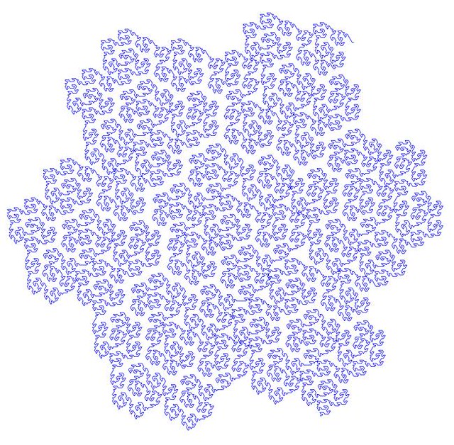
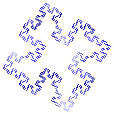
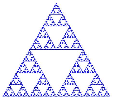
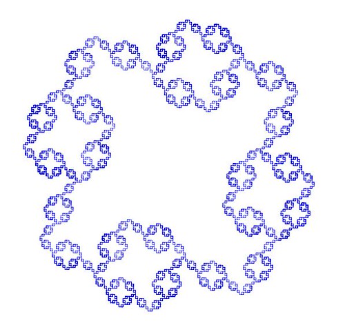
I would like to show a few more examples of beautiful curves generated with this technique, together with their generating axiom, rules and parameters. Feel free to click on each of the images below to download a larger version.

Note that any coding language with plotting capabilities should be able to tackle this project. I used once again tikz for , but this time with the tikzlibrary lindenmayersystems.

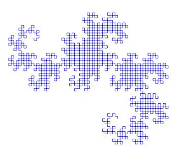
name : Dragon Curve axiom : X order : 11 step : 5pt angle : 90 rules : X -> X+YF+ Y -> -FX-Y	name : Gosper Space-filling Curve axiom : XF order : 5 step : 2pt angle : 60 rules : XF -> XF+YF++YF-XF--XFXF-YF+ YF -> -XF+YFYF++YF+XF--XF-YF
name : Quadric Koch Island axiom : F+F+F+F order : 4 step : 1pt angle : 90 rules : F -> F+F-F-FF+F+F-F	name : Sierpinski Arrowhead axiom : F order : 8 step : 3.5pt angle : 60 rules : G -> F+G+F F -> G-F-G
name : ? axiom : F+F+F+F order : 4 step : 2pt angle : 90 rules : F -> FF+F+F+F+F+F-F	name : ? axiom : F+F+F+F order : 4 step : 3pt angle : 90 rules : F -> FF+F+F+F+FF

Would you like to experiment a little with axioms, rules and parameters, and obtain some new pleasant curves with this method? If the mathematical properties of the fractal that they approximate are interesting enough, I bet you could attach your name to them. Like the astronomer that finds through her telescope a new object in the sky, or the zoologist that discover a new species of spider in the forest.

An Automatic Geometric Proof

We are familiar with that result that states that, on any given triangle, the circumcenter, centroid and orthocenter are always collinear. I would like to illustrate how to use Gröbner bases theory to prove that the incenter also belongs in the previous line, provided the triangle is isosceles.

We start, as usual, indicating that this property is independent of shifts, rotations or dilations, and therefore we may assume that the isosceles triangle has one vertex at , another vertex at and the third vertex at for some value In that case, we will need to work on the polynomial ring since we need the parameter free, the variables and are used to input the conditions for the circumcenter of the triangle, the variables and for centroid, and the variables and for the incenter (note that we do not need to use the orthocenter in this case).

We may obtain all six conditions by using sympy, as follows:

>>> import sympy
>>> from sympy import *
>>> A=Point(0,0)
>>> B=Point(1,0)
>>> s=symbols("s",real=True,positive=True)
>>> C=Point(1/2.,s)
>>> T=Triangle(A,B,C)
>>> T.circumcenter
Point(1/2, (4*s**2 - 1)/(8*s))
>>> T.centroid
Point(1/2, s/3)
>>> T.incenter
Point(1/2, s/(sqrt(4*s**2 + 1) + 1))

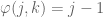
This translates into the following polynomials

(for circumcenter)
(for centroid)
(for incenter)

The hypothesis polynomial comes simply from asking whether the slope of the line through two of those centers is the same as the slope of the line through another choice of two centers; we could use then, for example, It only remains to compute the Gröbner basis of the ideal Let us use SageMath for this task:

sage: R.<s,x1,x2,x3,y1,y2,y3,z>=PolynomialRing(QQ,8,order='lex')
sage: h=[2*x1-1,8*r*y1-4*r**2+1,2*x2-1,3*y2-r,2*x3-1,(4*r*y3+1)**2-4*r**2-1]
sage: g=(x2-x1)*(y3-y1)-(x3-x1)*(y2-y1)
sage: I=R.ideal(1-z*g,*h)
sage: I.groebner_basis()
[1]

This proves the result.

Have a child, plant a tree, write a book

Or more importantly: rear your children to become nice people, water those trees, and make sure that your books make a good impact.

I recently enjoyed the rare pleasure of having a child (my first!) and publishing a book almost at the same time. Since this post belongs in my professional blog, I will exclusively comment on the latter: Learning SciPy for Numerical and Scientific Computing, published by Packt in a series of technical books focusing on Open Source software.

Keep in mind that the book is for a very specialized audience: not only do you need a basic knowledge of Python, but also a somewhat advanced command of mathematics/physics, and an interest in engineering or scientific applications. This is an excerpt of the detailed description of the monograph, as it reads in the publisher’s page:

It is essential to incorporate workflow data and code from various sources in order to create fast and effective algorithms to solve complex problems in science and engineering. Data is coming at us faster, dirtier, and at an ever increasing rate. There is no need to employ difficult-to-maintain code, or expensive mathematical engines to solve your numerical computations anymore. SciPy guarantees fast, accurate, and easy-to-code solutions to your numerical and scientific computing applications.

Learning SciPy for Numerical and Scientific Computing unveils secrets to some of the most critical mathematical and scientific computing problems and will play an instrumental role in supporting your research. The book will teach you how to quickly and efficiently use different modules and routines from the SciPy library to cover the vast scope of numerical mathematics with its simplistic practical approach that is easy to follow.

The book starts with a brief description of the SciPy libraries, showing practical demonstrations for acquiring and installing them on your system. This is followed by the second chapter which is a fun and fast-paced primer to array creation, manipulation, and problem-solving based on these techniques.

The rest of the chapters describe the use of all different modules and routines from the SciPy libraries, through the scope of different branches of numerical mathematics. Each big field is represented: numerical analysis, linear algebra, statistics, signal processing, and computational geometry. And for each of these fields all possibilities are illustrated with clear syntax, and plenty of examples. The book then presents combinations of all these techniques to the solution of research problems in real-life scenarios for different sciences or engineering — from image compression, biological classification of species, control theory, design of wings, to structural analysis of oxides.

The book is also being sold online in Amazon, where it has been received with pretty good reviews. I have found other random reviews elsewhere, with similar welcoming comments:

• Artificial Intelligence in Motion by Marcel Caraciolo
• The Endeavour, by John D. Cook

Stones, balances, matrices

Let’s examine an easy puzzle on finding the different stone by using a balance:

You have four stones identical in size and appearance, but one of them is heavier than the rest. You have a set of scales (a balance): how many weights do you need to determine which stone is the heaviest?

This is a trivial problem, but I will use it to illustrate different ideas, definitions, and the connection to linear algebra needed to answer the harder puzzles below. Let us start by solving it in the most natural way:

1. Enumerate each stone from 1 to 4.
2. Set stones 1 and 2 on the left plate; set stones 3 and 4 on the right plate. Since one of the stones is heavier, it will be in the plate that tips the balance. Let us assume this is the left plate.
3. Discard stones 3 and 4. Put stone 1 on the left plate; and stone 2 on the right plate. The plate that tips the balance holds the heaviest stone.

This solution finds the stone in two weights. It is what we call adaptive measures: each measure is determined by the result of the previous. This is a good point to introduce an algebraic scheme to code the solution.

• The weights matrix: This is a matrix with four columns (one for each stone) and two rows (one for each weight). The entries of this matrix can only be or depending whether a given stone is placed on the left plate , on the right plate or in neither plate For example, for the solution given above, the corresponding matrix would be
  
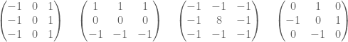
• The stones matrix: This is a square matrix with four rows and columns (one for each stone). Each column represents a different combination of stones, in such a way that the n-th column assumes that the heaviest stone is in the n-th position. The entries on this matrix indicate the weight of each stone. For example, if we assume that the heaviest stone weights b units, and each other stone weights a units, then the corresponding stones matrix is
  

Multiplying these two matrices, and looking at the sign of the entries of the resulting matrix, offers great insight on the result of the measures:

Note the columns of this matrix code the behavior of the measures:

• The column indicates that the balance tipped to the left in both measures (and therefore, the heaviest stone is the first one)
• The column indicates that the heaviest stone is the second one.
• Note that the other two measures can’t find the heaviest stone, since this matrix was designed to find adaptively a stone supposed to be either the first or the second.

Is it possible to design a solution to this puzzle that is not adaptive? Note the solution with two measures given (in algebraic form) below:

Since each column is different, it is trivial to decide after the experiment is done, which stone will be the heaviest. For instance, if the balance tips first to the right (-) and then to the left (+), the heaviest stone can only be the third one.

Let us make it a big harder: Same situation, but now we don’t know whether the stone that is different is heavier or lighter.

The solution above is no good: Since we are not sure whether b is greater or smaller than a, we would obtain two sign matrices which are virtually mirror images of each other.

and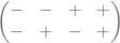

In this case, in the event of obtaining that the balance tips twice to the left: which would be the different stone? The first, which is heaviest, or the fourth, which is lightest? We cannot decide.

One possible solution to this situation involves taking one more measure. Look at the algebraic expression of the following example, to realize why:

or

In this case there is no room for confusion: if the balance tips three times to the same side, then the different stone is the first one (whether heavier or lighter). The other possibilities are also easily solvable: if the balance tips first to one side, then to the other, and then to the first side, then the different stone is the third one.

The reader will not be very surprised at this point to realize that three (non adaptive) measures are also enough to decide which stone is different (be it heavier or lighter) in a set of twelve similar stones. To design the solution, a good weight matrix with twelve columns and three rows need to be constructed. The trick here is to allow measures that balance both plates, which gives us more combinations with which to play. How would the reader design this matrix?

Buy my book!

Well, ok, it is not my book technically, but I am one of the authors of one of the chapters. And no, as far as I know, I don’t get a dime of the sales in concept of copyright or anything else.

As the title suggests (Modeling Nanoscale Imaging in Electron Microscopy), this book presents some recent advances that have been made using mathematical methods to resolve problems in electron microscopy. With improvements in hardware-based aberration software significantly expanding the nanoscale imaging capabilities of scanning transmission electron microscopes (STEM), these mathematical models can replace some labor intensive procedures used to operate and maintain STEMs. This book, the first in its field since 1998, covers relevant concepts such as super-resolution techniques (that’s my contribution!), special de-noising methods, application of mathematical/statistical learning theory, and compressed sensing.

We even got a nice review in Physics Today by Les Allen, no less!

Imaging with electrons, in particular scanning transmission electron microscopy (STEM), is now in widespread use in the physical and biological sciences. And its importance will only grow as nanotechnology and nano-Biology continue to flourish. Many applications of electron microscopy are testing the limits of current imaging capabilities and highlight the need for further technological improvements. For example, high throughput in the combinatorial chemical synthesis of catalysts demands automated imaging. The handling of noisy data also calls for new approaches, particularly because low electron doses are used for sensitive samples such as biological and organic specimens.

Modeling Nanoscale Imaging in Electron Microscopy addresses all those issues and more. Edited by Thomas Vogt and Peter Binev at the University of South Carolina (USC) and Wolfgang Dahmen at RWTH Aachen University in Germany, the book came out of a series of workshops organized by the Interdisciplinary Mathematics Institute and the NanoCenter at USC. Those sessions took the unusual but innovative approach of bringing together electron microscopists, engineers, physicists, mathematicians, and even a philosopher to discuss new strategies for image analysis in electron microscopy.

In six chapters, the editors tackle the ambitious challenge of bridging the gap between high-level applied mathematics and experimental electron microscopy. They have met the challenge admirably. I believe that high-resolution electron microscopy is at a point where it will benefit considerably from an influx of new mathematical approaches, daunting as they may seem; in that regard Modeling Nanoscale Imaging in Electron Microscopy is a major step forward. Some sections present a level of mathematical sophistication seldom encountered in the experimentally focused electron-microscopy literature.
The first chapter, by philosopher of science Michael Dickson, looks at the big picture by raising the question of how we perceive nano-structures and suggesting that a Kantian approach would be fruitful. The book then moves into a review of the application of STEM to nanoscale systems, by Nigel Browning, a leading experimentalist in the field, and other well-known experts. Using case studies, the authors show how beam-sensitive samples can be studied with high spatial resolution, provided one controls the beam dose and establishes the experimental parameters that allow for the optimum dose.

The third chapter, written by image-processing experts Sarah Haigh and Angus Kirkland, addresses the reconstruction, from atomic-resolution images, of the wave at the exit surface of a specimen. The exit surface wave is a fundamental quantity containing not only amplitude (image) information but also phase information that is often intimately related to the atomic-level structure of the specimen. The next two chapters, by Binev and other experts, are based on work carried out using the experimental and computational resources available at USC. Examples in chapter four address the mathematical foundations of compressed sensing as applied to electron microscopy, and in particular high-angle annular dark-field STEM. That emerging approach uses randomness to extract the essential content from low-information signals. Chapter five eloquently discusses the efficacy of analyzing several low-dose images with specially adapted digital-image-processing techniques that allow one to keep the cumulative electron dose low and still achieve acceptable resolution.

The book concludes with a wide-ranging discussion by mathematicians Amit Singer and Yoel Shkolnisky on the reconstruction of a three-dimensional object via projected data taken at random and initially unknown object orientations. The discussion is an extension of the authors’ globally consistent angular reconstitution approach for recovering the structure of a macromolecule using cryo-electron microscopy. That work is also applicable to the new generation of x-ray free-electron lasers, which have similar prospective applications, and illustrates nicely the importance of applied mathematics in the physical sciences.

Modeling Nanoscale Imaging in Electron Microscopy will be an important resource for graduate students and researchers in the area of high-resolution electron microscopy.

(Les J. Allen, Physics Today, Vol. 65 (5), May, 2012)

Table of contents	Preface	Sample chapter

Math still not the answer

I wrote a quick (but not very elegant) python script to retrieve locally enough data from www.metacritic.com for pattern recognition purposes. The main goal is to help me decide how much I will enjoy a movie, before watching it. I included the script at the end of the post, in case you want to try it yourself (and maybe improve it too!). It takes a while to complete, although it is quite entertaining to see its progress on screen. At the end, it provides with two lists of the same length: critics—a list of str containing the names of the critics; and scoredMovies—a list of dict containing, at index k, the evaluation of all the movies scored by the critic at index k in the previous list.

For example:

>>> critics[43]

‘James White’
>>> scoredMovies[43]

{‘hall-pass’: 60, ‘the-karate-kid’: 60, ‘the-losers’: 60,
‘the-avengers-2012’: 80, ‘the-other-guys’: 60, ‘shrek-forever-after’: 80,
‘the-lincoln-lawyer’: 80, ‘the-company-men’: 60, ‘jonah-hex’: 40,
‘arthur’: 60, ‘vampires-suck’: 20, ‘american-reunion’: 40,
‘footloose’: 60, ‘real-steel’: 60}

The number of scored films by critic varies: there are individuals that gave their opinion on a few dozen movies, and others that took the trouble to evaluate up to four thousand flicks! Note also that the names of the movies correspond with their web pages in www.metacritic.com. For example, to see what critics have to say about the “Karate Kid” and other relevant information online, point your browser to www.metacritic.com/movie/the-karate-kid. It also comes in very handy if there are several versions of a single title: Which “Karate Kid” does this score refer to, the one in the eighties, or Jackie Chan’s?

Feel free to download a copy of the resulting data [here] (note it is a large file: 1.6MB).

But the fact that we have that data stored locally allows us to gather that information with simple python commands, and perform many complex operations on it.

Edge detection: The Convolution Approach

Today I would like to show a very basic technique of detection based on simple convolution of an image with small kernels (masks). The purpose of these kernels is to enhance certain properties of the image at each pixel. What properties? Those that define what means to be an edge, in a differential calculus way—exactly as it was defined in the description of the Canny edge detector. The big idea is to assign to each pixel a numerical value that expresses its strength as an edge: positive if we suspect that such structure is present at that location, negative if not, and zero if the image is locally flat around that point. Masks can be designed so that they mimic the effect of differential operators, but these can be terribly complicated and give rise to large matrices.

The first approaches were performed with simple kernels. For example, Faler came up with the following four simple masks that emulate differentiation:

Note that, adding all the values of each matrix, one obtains zero. This is consistent with the third property required for our kernels: in the event of a locally flat area around a given pixel, convolution with any of these will offer a value of zero.

Read more…

So you want to be an Applied Mathematician

The way of the Applied Mathematician is one full of challenging and interesting problems. We thrive by association with the Pure Mathematician, and at the same time with the no-nonsense, hands-in, hard-core Engineer. But not everything is happy in Applied Mathematician land: every now and then, we receive the disregard of other professionals that mistake either our background, or our efficiency at attacking real-life problems.

I heard from a colleague (an Algebrist) complains that Applied Mathematicians did nothing but code solutions of partial differential equations in Fortran—his skewed view came up after a naïve observation of a few graduate students working on a project. The truth could not be further from this claim: we do indeed occasionally solve PDEs in Fortran—I give you that—and we are not ashamed to admit it. But before that job has to be addressed, we have gone through a great deal of thinking on how to better code this simple problem. And you would not believe the huge amount of deep Mathematics that are involved in this journey: everything from high-level Linear Algebra, Calculus of Variations, Harmonic Analysis, Differential Geometry, Microlocal Analysis, Functional Analysis, Dynamical Systems, the Theory of Distributions, etc. Not only are we familiar with the basic background on all those fields, but also we are supposed to be able to perform serious research on any of them at a given time.

My soon-to-be-converted Algebrist friend challenged me—not without a hint of smugness in his voice—to illustrate what was my last project at that time. This was one revolving around the idea of frames (think of it as redundant bases if you please), and needed proving a couple of inequalities involving sequences of functions in —spaces, which we attacked using a beautiful technique: Bellman functions. About ninety minutes later he conceded defeat in front of the board where the math was displayed. He promptly admitted that this was no Fortran code, and showed a newfound respect and reverence for the trade.

It doesn’t hurt either that the kind of problems that we attack are more likely to attract funding. And collaboration. And to be noticed in the press.

Alright, so some of you are sold already. What is the next step? I am assuming that at his point you own your Calculus, Analysis, Probability and Statistics, Linear Programming, Topology, Geometry, Physics and you are able to solve most known ODEs. From here, as with any other field, my recommendation is to slowly build a Batman belt: acquire and devour a sequence of books and scientific articles, until you are very familiar with their contents. When facing a new problem, you should be able to recall from your Batman belt what technique could work best, in which book(s) you could get some references, and how it has been used in the past for related problems.

Following these lines, I have included below an interesting collection with the absolutely essential books that, in my opinion, every Applied Mathematician should start studying:

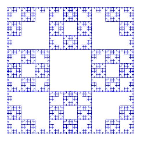
Where are the powers of two?

The following construction gives an interesting pairing map between the positive integers and the lattice of integer-valued points in the plane:

• Place at the origin.
• For each level populate the points of the plane on the square with vertices starting from at the position and going counter-clockwise.

  

After pairing enough positive integers on the lattice, pay attention to the powers of two: they all seem to be located on the same two horizontal lines: and

Is this statement true?

Geolocation

Recall the First Spherical Law of Cosines:

Given a unit sphere, a spherical triangle on the surface of the sphere is defined by the great circles connecting three points , , and on the sphere. If the lengths of these three sides are (from to (from to and (from to and the angle of the corner opposite is then

In any decent device and for most computer languages, this formula should give well-conditioned results down to distances as small as around three feet, and thus can be used to compute an accurate geodetic distance between two given points in the surface of the Earth (well, ok, assuming the Earth is a perfect sphere). The geodetic form of the law of cosines is rearranged from the canonical one so that the latitude can be used directly, rather than the colatitude, and reads as follows: Given points and with positions and respectively, the distance between the two points is given by the following formula.

where is the radius of the Earth in miles (well, ok, the average radius of the Earth…)

A nice application of this formula can be used for geolocation purposes, and I recently had the pleasure to assist a software company (thumb-mobile.com) to write such functionality for one of their clients.

Go to www.lizardsthicket.com in your mobile device, and click on “Find a Location.” This fires up the location services of your browser. When you accept, your latitude and longitude are tracked. After a fast, reliable and resource-efficient algorithm, the page offers the location of the restaurant from the Lizard’s chain that is closest to you. Simple, right?

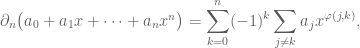
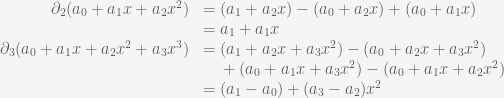
Boundary operators

Consider the vector space of polynomials with coefficients on a field , with the obvious sum of functions and scalar multiplication. For each , consider the subspaces spanned by polynomials of order ,

These subspaces have dimension Consider now for each the maps defined in the following way:

where if and otherwise.

Schematically, this can be written as follows

and it is not hard to prove that these maps are homeomorphisms of vector spaces over

Notice this interesting relationship between and

The kernel of and the image of are isomorphic!

The reader will surely have no trouble to show that this property is satisfied at all levels: As a consequence, for all

We say that a family of homomorphisms are boundary operators if for all If this is the case, then trivially The example above is a bit stronger, because of the isomorphism of both subspaces.

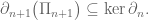
So this is the question I pose as today’s challenge:

Describe all boundary operators

Include a precise relationship between kernels and images of consecutive maps.