More on Lindenmayer Systems

We briefly explored Lindenmayer systems (or L-systems) in an old post: Toying with Basic Fractals. We quickly reviewed this method for creation of an approximation to fractals, and displayed an example (the Koch snowflake) based on tikz libraries.

I would like to show a few more examples of beautiful curves generated with this technique, together with their generating axiom, rules and parameters. Feel free to click on each of the images below to download a larger version.

Note that any coding language with plotting capabilities should be able to tackle this project. I used once again tikz for , but this time with the tikzlibrary lindenmayersystems.

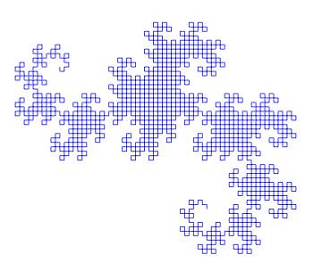
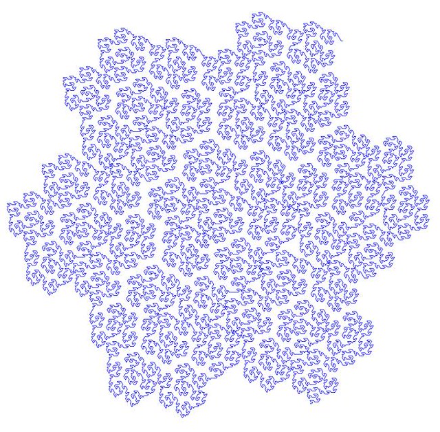
name : Dragon Curve axiom : X order : 11 step : 5pt angle : 90 rules : X -> X+YF+ Y -> -FX-Y	name : Gosper Space-filling Curve axiom : XF order : 5 step : 2pt angle : 60 rules : XF -> XF+YF++YF-XF--XFXF-YF+ YF -> -XF+YFYF++YF+XF--XF-YF
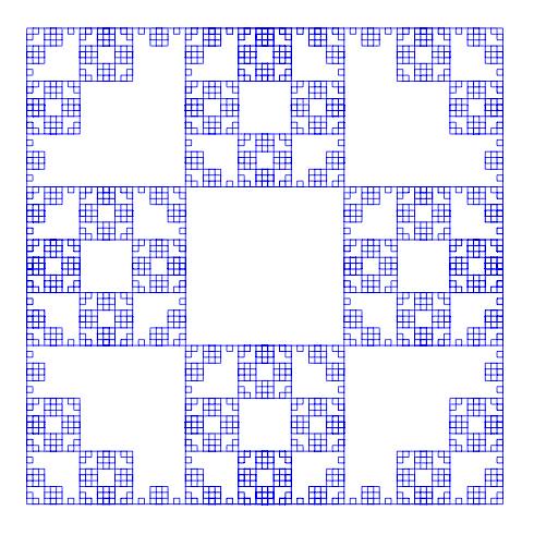
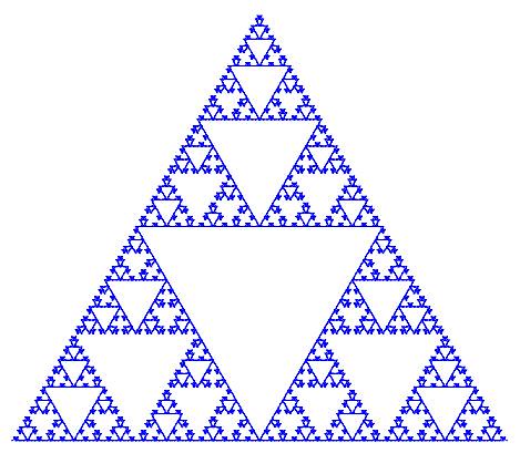
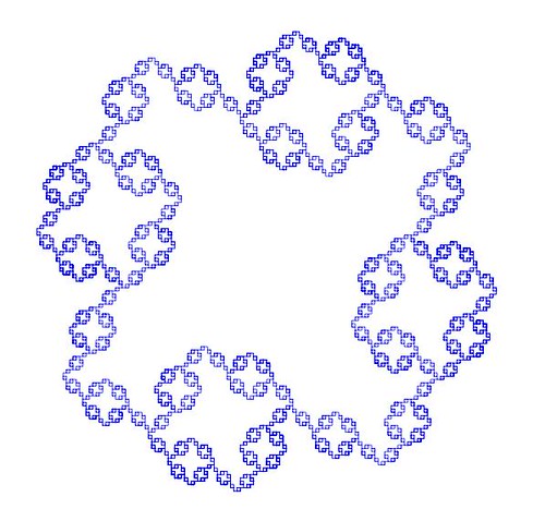
name : Quadric Koch Island axiom : F+F+F+F order : 4 step : 1pt angle : 90 rules : F -> F+F-F-FF+F+F-F	name : Sierpinski Arrowhead axiom : F order : 8 step : 3.5pt angle : 60 rules : G -> F+G+F F -> G-F-G
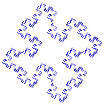
name : ? axiom : F+F+F+F order : 4 step : 2pt angle : 90 rules : F -> FF+F+F+F+F+F-F	name : ? axiom : F+F+F+F order : 4 step : 3pt angle : 90 rules : F -> FF+F+F+F+FF

Would you like to experiment a little with axioms, rules and parameters, and obtain some new pleasant curves with this method? If the mathematical properties of the fractal that they approximate are interesting enough, I bet you could attach your name to them. Like the astronomer that finds through her telescope a new object in the sky, or the zoologist that discover a new species of spider in the forest.