Archive
Searching (again!?) for the SS Central America
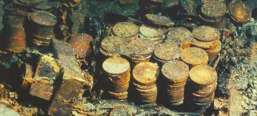
On Tuesday, September 8th 1857, the steamboat SS Central America left Havana at 9 AM for New York, carrying about 600 passengers and crew members. Inside of this vessel, there was stowed a very precious cargo: a set of manuscripts by John James Audubon, and three tons of gold bars and coins. The manuscripts documented an expedition through the yet uncharted southwestern United States and California, and contained 200 sketches and paintings of its wildlife. The gold, fruit of many years of prospecting and mining during the California Gold Rush, was meant to start anew the lives of many of the passengers aboard.
On the 9th, the vessel ran into a storm which developed into a hurricane. The steamboat endured four hard days at sea, and by Saturday morning the ship was doomed. The captain arranged to have women and children taken off to the brig Marine, which offered them assistance at about noon. In spite of the efforts of the remaining crew and passengers to save the ship, the inevitable happened at about 8 PM that same day. The wreck claimed the lives of 425 men, and carried the valuable cargo to the bottom of the sea.
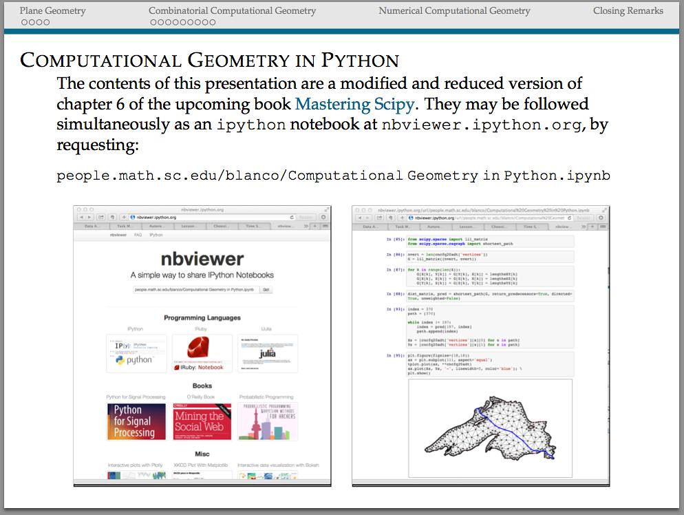
It was not until late 1980s that technology allowed recovery of shipwrecks at deep sea. But no technology would be of any help without an accurate location of the site. In the following paragraphs we would like to illustrate the power of the scipy stack by performing a simple simulation, that ultimately creates a dataset of possible locations for the wreck of the SS Central America, and mines the data to attempt to pinpoint the most probable target.
We simulate several possible paths of the steamboat (say 10,000 randomly generated possibilities), between 7:00 AM on Saturday, and 13 hours later, at 8:00 pm on Sunday. At 7:00 AM on that Saturday the ship’s captain, William Herndon, took a celestial fix and verbally relayed the position to the schooner El Dorado. The fix was 31º25′ North, 77º10′ West. Because the ship was not operative at that point—no engine, no sails—, for the next thirteen hours its course was solely subjected to the effect of ocean current and winds. With enough information, it is possible to model the drift and leeway on different possible paths.
Book presentation at the USC Python Users Group
Areas of Mathematics
For one of my upcoming talks I am trying to include an exhaustive mindmap showing the different areas of Mathematics, and somehow, how they relate to each other. Most of the information I am using has been processed from years of exposure in the field, and a bit of help from Wikipedia.

But I am not entirely happy with what I see: my lack of training in the area of Combinatorics results in a rather dry treatment of that part of the mindmap, for example. I am afraid that the same could be told about other parts of the diagram. Any help from the reader to clarify and polish this information will be very much appreciated.
And as a bonus, I included a script to generate the diagram with the aid of the tikz libraries.
\tikzstyle{level 2 concept}+=[sibling angle=40]
\begin{tikzpicture}[scale=0.49, transform shape]
  \path[mindmap,concept color=black,text=white]
    node[concept] {Pure Mathematics} [clockwise from=45]
      child[concept color=DeepSkyBlue4]{
        node[concept] {Analysis} [clockwise from=180]
          child {
            node[concept] {Multivariate \& Vector Calculus}
              [clockwise from=120]
              child {node[concept] {ODEs}}}
              child { node[concept] {Functional Analysis}}
              child { node[concept] {Measure Theory}}
              child { node[concept] {Calculus of Variations}}
              child { node[concept] {Harmonic Analysis}}
              child { node[concept] {Complex Analysis}}
              child { node[concept] {Stochastic Analysis}}
              child { node[concept] {Geometric Analysis}
                [clockwise from=-40]
                child {node[concept] {PDEs}}}}
          child[concept color=black!50!green, grow=-40]{
            node[concept] {Combinatorics} [clockwise from=10]
              child {node[concept] {Enumerative}}
              child {node[concept] {Extremal}}
              child {node[concept] {Graph Theory}}}
          child[concept color=black!25!red, grow=-90]{
            node[concept] {Geometry} [clockwise from=-30]
              child {node[concept] {Convex Geometry}}
              child {node[concept] {Differential Geometry}}
              child {node[concept] {Manifolds}}
              child {node[concept,color=black!50!green!50!red,text=white] {Discrete Geometry}}
              child {
                node[concept] {Topology} [clockwise from=-150]
                  child {node [concept,color=black!25!red!50!brown,text=white]
                    {Algebraic Topology}}}}
          child[concept color=brown,grow=140]{
            node[concept] {Algebra} [counterclockwise from=70]
              child {node[concept] {Elementary}}
              child {node[concept] {Number Theory}}
              child {node[concept] {Abstract} [clockwise from=180]
                child {node[concept,color=red!25!brown,text=white] {Algebraic Geometry}}}
              child {node[concept] {Linear}}}
    node[extra concept,concept color=black] at (200:5) {Applied Mathematics}
      child[grow=145,concept color=black!50!yellow] {
        node[concept] {Probability} [clockwise from=180]
          child {node[concept] {Stochastic Processes}}}
      child[grow=175,concept color=black!50!yellow] {node[concept] {Statistics}}
      child[grow=205,concept color=black!50!yellow] {node[concept] {Numerical Analysis}}
      child[grow=235,concept color=black!50!yellow] {node[concept] {Symbolic Computation}};
\end{tikzpicture}
More on Lindenmayer Systems
We briefly explored Lindenmayer systems (or L-systems) in an old post: Toying with Basic Fractals. We quickly reviewed this method for creation of an approximation to fractals, and displayed an example (the Koch snowflake) based on tikz libraries.
I would like to show a few more examples of beautiful curves generated with this technique, together with their generating axiom, rules and parameters. Feel free to click on each of the images below to download a larger version.
Note that any coding language with plotting capabilities should be able to tackle this project. I used once again tikz for , but this time with the tikzlibrary lindenmayersystems.
Would you like to experiment a little with axioms, rules and parameters, and obtain some new pleasant curves with this method? If the mathematical properties of the fractal that they approximate are interesting enough, I bet you could attach your name to them. Like the astronomer that finds through her telescope a new object in the sky, or the zoologist that discover a new species of spider in the forest.
Some results related to the Feuerbach Point
Given a triangle the circle that goes through the midpoints of each side,
is called the Feuerbach circle. It has very surprising properties:
- It also goes through the feet of the heights, points
- If
denotes the orthocenter of the triangle, then the Feuerbach circle also goes through the midpoints of the segments
For this reason, the Feuerbach circle is also called the nine-point circle.
- The center of the Feuerbach circle is the midpoint between the orthocenter and circumcenter of the triangle.
- The area of the circumcircle is precisely four times the area of the Feuerbach circle.
Most of these results are easily shown with sympy without the need to resort to Gröbner bases or Ritt-Wu techniques. As usual, we realize that the properties are independent of rotation, translation or dilation, and so we may assume that the vertices of the triangle are and
for some positive parameters
To prove the last statement, for instance we may issue the following:
>>> import sympy
>>> from sympy import *
>>> A=Point(0,0)
>>> B=Point(1,0)
>>> r,s=var('r,s')
>>> C=Point(r,s)
>>> D=Segment(A,B).midpoint
>>> E=Segment(B,C).midpoint
>>> F=Segment(A,C).midpoint
>>> simplify(Triangle(A,B,C).circumcircle.area/Triangle(D,E,F).circumcircle.area)
4
But probably the most amazing property of the nine-point circle, is the fact that it is tangent to the incircle of the triangle. With exception of the case of equilateral triangles, both circles intersect only at one point: the so-called Feuerbach point.
An Automatic Geometric Proof
We are familiar with that result that states that, on any given triangle, the circumcenter, centroid and orthocenter are always collinear. I would like to illustrate how to use Gröbner bases theory to prove that the incenter also belongs in the previous line, provided the triangle is isosceles.
We start, as usual, indicating that this property is independent of shifts, rotations or dilations, and therefore we may assume that the isosceles triangle has one vertex at , another vertex at
and the third vertex at
for some value
In that case, we will need to work on the polynomial ring
since we need the parameter
free, the variables
and
are used to input the conditions for the circumcenter of the triangle, the variables
and
for centroid, and the variables
and
for the incenter (note that we do not need to use the orthocenter in this case).
We may obtain all six conditions by using sympy, as follows:
>>> import sympy
>>> from sympy import *
>>> A=Point(0,0)
>>> B=Point(1,0)
>>> s=symbols("s",real=True,positive=True)
>>> C=Point(1/2.,s)
>>> T=Triangle(A,B,C)
>>> T.circumcenter
Point(1/2, (4*s**2 - 1)/(8*s))
>>> T.centroid
Point(1/2, s/3)
>>> T.incenter
Point(1/2, s/(sqrt(4*s**2 + 1) + 1))
This translates into the following polynomials
The hypothesis polynomial comes simply from asking whether the slope of the line through two of those centers is the same as the slope of the line through another choice of two centers; we could use then, for example, It only remains to compute the Gröbner basis of the ideal
Let us use SageMath for this task:
sage: R.<s,x1,x2,x3,y1,y2,y3,z>=PolynomialRing(QQ,8,order='lex')
sage: h=[2*x1-1,8*r*y1-4*r**2+1,2*x2-1,3*y2-r,2*x3-1,(4*r*y3+1)**2-4*r**2-1]
sage: g=(x2-x1)*(y3-y1)-(x3-x1)*(y2-y1)
sage: I=R.ideal(1-z*g,*h)
sage: I.groebner_basis()
[1]
This proves the result.
Have a child, plant a tree, write a book
Or more importantly: rear your children to become nice people, water those trees, and make sure that your books make a good impact.
I recently enjoyed the rare pleasure of having a child (my first!) and publishing a book almost at the same time. Since this post belongs in my professional blog, I will exclusively comment on the latter: Learning SciPy for Numerical and Scientific Computing, published by Packt in a series of technical books focusing on Open Source software.
Keep in mind that the book is for a very specialized audience: not only do you need a basic knowledge of Python, but also a somewhat advanced command of mathematics/physics, and an interest in engineering or scientific applications. This is an excerpt of the detailed description of the monograph, as it reads in the publisher’s page:
It is essential to incorporate workflow data and code from various sources in order to create fast and effective algorithms to solve complex problems in science and engineering. Data is coming at us faster, dirtier, and at an ever increasing rate. There is no need to employ difficult-to-maintain code, or expensive mathematical engines to solve your numerical computations anymore. SciPy guarantees fast, accurate, and easy-to-code solutions to your numerical and scientific computing applications.
Learning SciPy for Numerical and Scientific Computing unveils secrets to some of the most critical mathematical and scientific computing problems and will play an instrumental role in supporting your research. The book will teach you how to quickly and efficiently use different modules and routines from the SciPy library to cover the vast scope of numerical mathematics with its simplistic practical approach that is easy to follow.
The book starts with a brief description of the SciPy libraries, showing practical demonstrations for acquiring and installing them on your system. This is followed by the second chapter which is a fun and fast-paced primer to array creation, manipulation, and problem-solving based on these techniques.
The rest of the chapters describe the use of all different modules and routines from the SciPy libraries, through the scope of different branches of numerical mathematics. Each big field is represented: numerical analysis, linear algebra, statistics, signal processing, and computational geometry. And for each of these fields all possibilities are illustrated with clear syntax, and plenty of examples. The book then presents combinations of all these techniques to the solution of research problems in real-life scenarios for different sciences or engineering — from image compression, biological classification of species, control theory, design of wings, to structural analysis of oxides.
The book is also being sold online in Amazon, where it has been received with pretty good reviews. I have found other random reviews elsewhere, with similar welcoming comments:
- Artificial Intelligence in Motion by Marcel Caraciolo
- The Endeavour, by John D. Cook
Which one is the fake?

|

|

|
“Crab on its back” | “Willows at sunset” | “Still life: Potatoes in a yellow dish” |
Buy my book!
Well, ok, it is not my book technically, but I am one of the authors of one of the chapters. And no, as far as I know, I don’t get a dime of the sales in concept of copyright or anything else.
As the title suggests (Modeling Nanoscale Imaging in Electron Microscopy), this book presents some recent advances that have been made using mathematical methods to resolve problems in electron microscopy. With improvements in hardware-based aberration software significantly expanding the nanoscale imaging capabilities of scanning transmission electron microscopes (STEM), these mathematical models can replace some labor intensive procedures used to operate and maintain STEMs. This book, the first in its field since 1998, covers relevant concepts such as super-resolution techniques (that’s my contribution!), special de-noising methods, application of mathematical/statistical learning theory, and compressed sensing.
We even got a nice review in Physics Today by Les Allen, no less!
Imaging with electrons, in particular scanning transmission electron microscopy (STEM), is now in widespread use in the physical and biological sciences. And its importance will only grow as nanotechnology and nano-Biology continue to flourish. Many applications of electron microscopy are testing the limits of current imaging capabilities and highlight the need for further technological improvements. For example, high throughput in the combinatorial chemical synthesis of catalysts demands automated imaging. The handling of noisy data also calls for new approaches, particularly because low electron doses are used for sensitive samples such as biological and organic specimens.
Modeling Nanoscale Imaging in Electron Microscopy addresses all those issues and more. Edited by Thomas Vogt and Peter Binev at the University of South Carolina (USC) and Wolfgang Dahmen at RWTH Aachen University in Germany, the book came out of a series of workshops organized by the Interdisciplinary Mathematics Institute and the NanoCenter at USC. Those sessions took the unusual but innovative approach of bringing together electron microscopists, engineers, physicists, mathematicians, and even a philosopher to discuss new strategies for image analysis in electron microscopy.
In six chapters, the editors tackle the ambitious challenge of bridging the gap between high-level applied mathematics and experimental electron microscopy. They have met the challenge admirably. I believe that high-resolution electron microscopy is at a point where it will benefit considerably from an influx of new mathematical approaches, daunting as they may seem; in that regard Modeling Nanoscale Imaging in Electron Microscopy is a major step forward. Some sections present a level of mathematical sophistication seldom encountered in the experimentally focused electron-microscopy literature.
The first chapter, by philosopher of science Michael Dickson, looks at the big picture by raising the question of how we perceive nano-structures and suggesting that a Kantian approach would be fruitful. The book then moves into a review of the application of STEM to nanoscale systems, by Nigel Browning, a leading experimentalist in the field, and other well-known experts. Using case studies, the authors show how beam-sensitive samples can be studied with high spatial resolution, provided one controls the beam dose and establishes the experimental parameters that allow for the optimum dose.The third chapter, written by image-processing experts Sarah Haigh and Angus Kirkland, addresses the reconstruction, from atomic-resolution images, of the wave at the exit surface of a specimen. The exit surface wave is a fundamental quantity containing not only amplitude (image) information but also phase information that is often intimately related to the atomic-level structure of the specimen. The next two chapters, by Binev and other experts, are based on work carried out using the experimental and computational resources available at USC. Examples in chapter four address the mathematical foundations of compressed sensing as applied to electron microscopy, and in particular high-angle annular dark-field STEM. That emerging approach uses randomness to extract the essential content from low-information signals. Chapter five eloquently discusses the efficacy of analyzing several low-dose images with specially adapted digital-image-processing techniques that allow one to keep the cumulative electron dose low and still achieve acceptable resolution.
The book concludes with a wide-ranging discussion by mathematicians Amit Singer and Yoel Shkolnisky on the reconstruction of a three-dimensional object via projected data taken at random and initially unknown object orientations. The discussion is an extension of the authors’ globally consistent angular reconstitution approach for recovering the structure of a macromolecule using cryo-electron microscopy. That work is also applicable to the new generation of x-ray free-electron lasers, which have similar prospective applications, and illustrates nicely the importance of applied mathematics in the physical sciences.
Modeling Nanoscale Imaging in Electron Microscopy will be an important resource for graduate students and researchers in the area of high-resolution electron microscopy.
(Les J. Allen, Physics Today, Vol. 65 (5), May, 2012)

|

|

|
| Table of contents | Preface | Sample chapter |
Sometimes Math is not the answer
 I would love to stand corrected in this case, though. Let me explain first the reason behind this claim—It will take a minute, so bear with me:
Say there is a new movie released, and you would like to know how good it is, or whether you and your partner will enjoy watching it together. There are plenty of online resources out there that will give you enough information to make an educated opinion but, let’s face it, you will not have the complete picture unless you actually go see the movie (sorry for the pun).
For example, I fell for “The Blair Witch Project:” their amazing advertising campaign promised me thrill and originality. On top of that, the averaged evaluation of many movie critics that had access to previews claimed that this was a flick not to be missed… Heck, I even bought the DVD for my sister before even watching it!—She and I have a similar taste with respect to movies. The disappointment was, obviously, epic. Before that, and many a time afterwards, I have tripped over the same stone. If nothing else, I learned not to trust commercials and sneak previews any more (“Release the Kraken!
,” anyone?)
The only remaining resource should then be the advice of the knowledgeable movie critics—provided you trust on their integrity, that is. Then it hit me: My taste in movies, so similar to my sister’s, could be completely different to that of the “average critic”. Being that the case, why would I trust what a bunch of experts have to say? The mathematician in me took over, and started planning a potential algorithm:
What if?

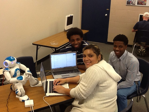
Sara, Spencer and Cam (left to right) discussing their projects in office hour
“What if?” is a truly powerful question. It is the question that separates the child from the adult; the student from the professional. Average students will go through the motions of a course and ask themselves many times: “What is the point of all this?” On the other hand, the notable students on their way to excellence will ask themselves: “How can I profit from this?” It is these inquiring minds who make it at the end: they are a pleasure to work with, they have the drive and the passion to get the job done, enjoy the process, and they are more likely to give their future employers more of their time in pursue of solutions—not because there is monetary or status gain alone, but because their commitment is only matched with their skill and curiosity.
It is a thrill to witness your own students pose that “What if?” question to themselves, and take steps to accomplish that little dream with the knowledge obtained in class. This semester, I had been blessed with a group of extremely talented people in all my different teaching assignments—especially those in my course on elementary differential equations.
Edge detection: The Convolution Approach
Today I would like to show a very basic technique of detection based on simple convolution of an image with small kernels (masks). The purpose of these kernels is to enhance certain properties of the image at each pixel. What properties? Those that define what means to be an edge, in a differential calculus way—exactly as it was defined in the description of the Canny edge detector. The big idea is to assign to each pixel a numerical value that expresses its strength as an edge: positive if we suspect that such structure is present at that location, negative if not, and zero if the image is locally flat around that point. Masks can be designed so that they mimic the effect of differential operators, but these can be terribly complicated and give rise to large matrices.
The first approaches were performed with simple kernels. For example, Faler came up with the following four simple masks that emulate differentiation:
Note that, adding all the values of each matrix, one obtains zero. This is consistent with the third property required for our kernels: in the event of a locally flat area around a given pixel, convolution with any of these will offer a value of zero.
OpArt
 OpArt is, by definition, a style of visual art based upon optical illusions. Let it be a painting, a photograph or any other mean, the objective of this style is to play with the interaction of what you see, and what it really is. A classical OpArt piece involves confusion by giving impression of movement, impossible solids, hidden images, conflicting patterns, warping, etc. And of course, Mathematics is a perfect vehicle to study—and even perform—this form of art.
In this post I would like to show an example of how to use trivial mathematics to implement a well-known example (shown above) in with the tikz package, and leave as homework another more interesting example.
Observe first the image above: the optical effect arises when conflicting concentric squares change the direction of their patterns. You may think that the color is the culprit of this effect but, as you will see below, it is only the relationship between the pure black-and-white patterns what produces the impression of movement.
So you want to be an Applied Mathematician
The way of the Applied Mathematician is one full of challenging and interesting problems. We thrive by association with the Pure Mathematician, and at the same time with the no-nonsense, hands-in, hard-core Engineer. But not everything is happy in Applied Mathematician land: every now and then, we receive the disregard of other professionals that mistake either our background, or our efficiency at attacking real-life problems.
I heard from a colleague (an Algebrist) complains that Applied Mathematicians did nothing but code solutions of partial differential equations in Fortran—his skewed view came up after a naïve observation of a few graduate students working on a project. The truth could not be further from this claim: we do indeed occasionally solve PDEs in Fortran—I give you that—and we are not ashamed to admit it. But before that job has to be addressed, we have gone through a great deal of thinking on how to better code this simple problem. And you would not believe the huge amount of deep Mathematics that are involved in this journey: everything from high-level Linear Algebra, Calculus of Variations, Harmonic Analysis, Differential Geometry, Microlocal Analysis, Functional Analysis, Dynamical Systems, the Theory of Distributions, etc. Not only are we familiar with the basic background on all those fields, but also we are supposed to be able to perform serious research on any of them at a given time.
My soon-to-be-converted Algebrist friend challenged me—not without a hint of smugness in his voice—to illustrate what was my last project at that time. This was one revolving around the idea of frames (think of it as redundant bases if you please), and needed proving a couple of inequalities involving sequences of functions in —spaces, which we attacked using a beautiful technique: Bellman functions. About ninety minutes later he conceded defeat in front of the board where the math was displayed. He promptly admitted that this was no Fortran code, and showed a newfound respect and reverence for the trade.
It doesn’t hurt either that the kind of problems that we attack are more likely to attract funding. And collaboration. And to be noticed in the press.
Alright, so some of you are sold already. What is the next step? I am assuming that at his point you own your Calculus, Analysis, Probability and Statistics, Linear Programming, Topology, Geometry, Physics and you are able to solve most known ODEs. From here, as with any other field, my recommendation is to slowly build a Batman belt: acquire and devour a sequence of books and scientific articles, until you are very familiar with their contents. When facing a new problem, you should be able to recall from your Batman belt what technique could work best, in which book(s) you could get some references, and how it has been used in the past for related problems.
Following these lines, I have included below an interesting collection with the absolutely essential books that, in my opinion, every Applied Mathematician should start studying:
Geolocation
Recall the First Spherical Law of Cosines:
Given a unit sphere, a spherical triangle on the surface of the sphere is defined by the great circles connecting three points
,
, and
on the sphere. If the lengths of these three sides are
(from
to

(from
to
and
(from
to
and the angle of the corner opposite
is
then
In any decent device and for most computer languages, this formula should give well-conditioned results down to distances as small as around three feet, and thus can be used to compute an accurate geodetic distance between two given points in the surface of the Earth (well, ok, assuming the Earth is a perfect sphere). The geodetic form of the law of cosines is rearranged from the canonical one so that the latitude can be used directly, rather than the colatitude, and reads as follows: Given points and
with positions
and
respectively, the distance
between the two points is given by the following formula.
where is the radius of the Earth in miles (well, ok, the average radius of the Earth…)
A nice application of this formula can be used for geolocation purposes, and I recently had the pleasure to assist a software company (thumb-mobile.com) to write such functionality for one of their clients.
 |
 |
 |
Go to www.lizardsthicket.com in your mobile device, and click on “Find a Location.” This fires up the location services of your browser. When you accept, your latitude and longitude are tracked. After a fast, reliable and resource-efficient algorithm, the page offers the location of the restaurant from the Lizard’s chain that is closest to you. Simple, right?
Apollonian gaskets and circle inversion fractals
Recall the definition of an iterated function system (IFS), and how on occasion, their attractors are fractal sets. What happens when we allow more general functions instead of mere affine maps?

The key to the design of this amazing fractal is in the notion of limit sets of circle inversions.
Unusual dice
 I heard of this problem from Justin James in his TechRepublic post My First IronRuby Application. He tried this fun problem as a toy example to brush up his skills in ruby:
Roll simultaneously a hundred 100-sided dice, and add the resulting values. The set of possible outcomes is, of course, Note that there is only one way to obtain the outcome 100—all dice showing a 1. There is also only one way to obtain the outcome 10000—all dice showing 100. For the outcome 101, there are exactly 100 different ways to obtain it: all dice except one show a 1, and one die shows a 2. The follow-up question is:
Write a (fast) script that computes the different ways in which we can obtain each of the possible outcomes.
Wavelets in sage
There are no native wavelet packages in sage. But there is a great module in python that contains, among other things, forward and inverse discrete wavelet transforms (for one and two dimensions). It comes bundled with seventy-six wavelet filters, and allows support to build your own! The name is PyWavelets, written by Tariq Rashid, and can be retrieved from pypi.python.org/pypi/PyWavelets. In order to install it in sage, take the following steps:
Edge detection: The Scale Space Theory
Consider an image as a bounded function with no smoothness or structure assumptions a priori. Most relevant information of a given image is contained in the contours of the mapped objects: Think for example of a bright object against a dark background—the area where these two meet presents a curve where the intensity
varies strongly. This is what we refer to as an “edge.”

Initially, we may consider the process of detection of an edge by the simple computation of the gradient This gradient should have a large intensity
and a direction
which indicates the perpendicular to the curve. It therefore looks sound to simply compute the gradient of
and choose the points where these values are large. This conclusion is a bit unrealistic for two reasons:
- The points where the gradient is larger than a given threshold are open sets, and thus don’t have the structure of curves.
- Large gradient may arise in certain locations of the image due to tiny oscillations or noise, but completely unrelated to the objects being mapped. As a matter of fact, there is no reason to assume the existence or computability of any gradient at all in a given digital image.
Voronoi mosaics
While looking for ideas to implement voronoi in sage, I stumbled upon a beautiful paper written by a group of japanese computer graphic professionals from the universities of Hokkaido and Tokyo: A Method for Creating Mosaic Images Using Voronoi Diagrams. The first step of their algorithm is simple yet brilliant: Start with any given image, and superimpose an hexagonal tiling of the plane. By a clever approximation scheme, modify the tiling to become a voronoi diagram that adaptively minimizes some approximation error. As a consequence, the resulting voronoi diagram is somehow adapted to the desired contours of the original image.
 |
 |
 |
 |
| (Fig. 1) | (Fig. 2) | (Fig. 3) | (Fig. 4) |
In a second step, they manually adjust the Voronoi image interactively by moving, adding, or deleting sites. They also take the liberty of adding visual effects by hand: emphasizing the outlines and color variations in each Voronoi region, so they look like actual pieces of stained glass (Fig. 4).
Image Processing with numpy, scipy and matplotlibs in sage
In this post, I would like to show how to use a few different features of numpy, scipy and matplotlibs to accomplish a few basic image processing tasks: some trivial image manipulation, segmentation, obtaining of structural information, etc. An excellent way to show a good set of these techniques is by working through a complex project. In this case, I have chosen the following:
Given a HAADF-STEM micrograph of a bronze-type Niobium Tungsten oxide
(left), find a script that constructs a good approximation to its structural model (right).
Courtesy of ETH Zurich
For pedagogical purposes, I took the following approach to solving this problem:
- Segmentation of the atoms by thresholding and morphological operations.
- Connected component labeling to extract each single atom for posterior examination.
- Computation of the centers of mass of each label identified as an atom. This presents us with a lattice of points in the plane that shows a first insight in the structural model of the oxide.
- Computation of Delaunay triangulation and Voronoi diagram of the previous lattice of points. The combination of information from these two graphs will lead us to a decent (approximation to the actual) structural model of our sample.
Let us proceed in this direction:
Super-Resolution Micrograph Reconstruction by Nonlocal-Means Applied to HAADF-STEM
We outline a new systematic approach to extracting high-resolution information from HAADF–STEM images which will be beneficial to the characterization of beam sensitive materials. The idea is to treat several, possibly many low electron dose images with specially adapted digital image processing concepts at a minimum allowable spatial resolution. Our goal is to keep the overall cumulative electron dose as low as possible while still staying close to an acceptable level of physical resolution. We wrote a letter indicating the main conceptual imaging concepts and restoration methods that we believe are suitable for carrying out such a program and, in particular, allow one to correct special acquisition artifacts which result in blurring, aliasing, rastering distortions and noise.
Below you can find a preprint of that document and a pdf presentation about this work that I gave in the SEMS 2010 meeting, in Charleston, SC. Click on either image to download.
 |
 |
The Nonlocal-means Algorithm
The nonlocal-means algorithm [Buades, Coll, Morel] was designed to perform noise reduction on digital images, while preserving the main geometrical configurations, as well as finer structures, details and texture. The algorithm is consistent under the condition that one can find many samples of every image detail within the same image.
 |
 |
 |
| Barbara | Noise added, std=30 | Denoised image, h=93 |
The algorithm has the following closed form: Given a finite grid of the form
for some compact set
, a signal
, and a family of windows
satisfying the conditions
for all
.
- If
, then
,
the nonlocal-means operator with filtering parameter
, is defined by
where the weights are defined by
Here, denotes a patch of the image
supported on the window
.
Notice that the similarity check between patches is nothing but a simple Gaussian weighted Euclidean distance, which accounts for difference of grayscales alone. Efros and Leung prove that this distance is a reliable measure for the comparison of texture patches, and at the same time copes very well with additive white noise; in particular, if and
are respectively the noisy and original images, and
is the noise variance, then the most similar patches in the noisy image are also expected to be the most similar in the original:
Wavelet Coefficients
To aid in my understanding of wavelets, during the first months I started studying this subject I wrote a couple of scripts to both compute wavelet coefficients of a given pgm gray-scale image (the decoding script), and recover an approximation to the original image from a subset of those coefficients (the coding script). I used OCaml, a multi-paradigm language: imperative, functional and object-oriented.
The decoding script uses the easiest wavelets possible: the Haar functions. As it was suggested in the article “Fast wavelet techniques for near-optimal image processing“, by R. DeVore and B.J. Lucier, rather than computing the actual raw wavelet coefficients, one computes instead a related integer value (a code). The coding script interprets those integer values and modifies them appropriately to obtain the actual coefficients. The storage of the integers is performed using Huffman trees, but I used a very simple one, not designed for speed or optimization in any way.
Following a paper by A.Chambolle, R.DeVore, N.Y.Lee and B.Lucier, “Non-linear wavelet image processing: Variational problems, compression and noise removal through wavelet shrinkage“, these scripts were used in two experiments later on: computation of the smoothness of an image, and removal of Gaussian white noise by the wavelet shrinkage method proposed by Donoho and Johnstone in the early 90’s.
 |
 |
 |
 |
 |
 |
 |
 |
Progressive reconstruction of a grey-scale image of size with the largest (in absolute value)
coefficients,
Modeling the Impact of Ebola and Bushmeat Hunting on Western Lowland Gorillas
In May 2003, together with fellow Mathematician Stephanie Gruver, Statistician Young-Ju Kim, and Forestry Engineer Carol Rizkalla, we worked on this little project to apply ideas from Dynamical Systems to an epidemiology model of the Ebola hemorrhagic fever in the Republic of Congo. The manuscript ebola/root.pdf is a first draft, and contains most of the mathematics behind the study. Carol worked in a less-math-more-biology version: ebola/Ecohealth.pdf “Modeling the Impact of Ebola and Bushmeat Hunting on Western Lowland Gorillas,” and presented it to EcoHealth, where it has been published (June 2007). She also prepared a poster for the Sigma-Xi competition: Click on the image below to retrieve a PowerPoint version of it.
Triangulations
As part of a project developed by Professor Bradley J. Lucier, to code a PDE solver written in scheme, I worked in some algorithms to perform “good triangulations” of polygons with holes (“good triangulations” meaning here, those where all the triangles have their three angles as close to 60º as possible). I obtained the necessary theoretical background and coding strategies from the following references:
- Mark de Berg et al., “Computational Geometry by Example.“
- Francis Chin and Cao An Wang, “Finding the Constrained Delaunay Triangulation and Constrained Voronoi Diagram of a simple Polygon in Linear Time.“
- Joseph O’Rourke, “Computational Geometry in C.“
- Jim Ruppert, “A Delaunay Refinement Algorithm for Quality 2-dimensional Mesh Generation.“
