Areas of Mathematics

For one of my upcoming talks I am trying to include an exhaustive mindmap showing the different areas of Mathematics, and somehow, how they relate to each other. Most of the information I am using has been processed from years of exposure in the field, and a bit of help from Wikipedia.

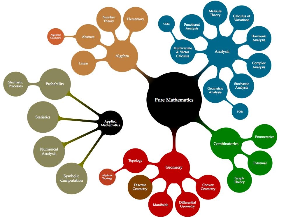
But I am not entirely happy with what I see: my lack of training in the area of Combinatorics results in a rather dry treatment of that part of the mindmap, for example. I am afraid that the same could be told about other parts of the diagram. Any help from the reader to clarify and polish this information will be very much appreciated.

And as a bonus, I included a script to generate the diagram with the aid of the tikz libraries.

\tikzstyle{level 2 concept}+=[sibling angle=40]
\begin{tikzpicture}[scale=0.49, transform shape]
  \path[mindmap,concept color=black,text=white]
    node[concept] {Pure Mathematics} [clockwise from=45]
      child[concept color=DeepSkyBlue4]{
        node[concept] {Analysis} [clockwise from=180]
          child { 
            node[concept] {Multivariate \& Vector Calculus}
              [clockwise from=120]
              child {node[concept] {ODEs}}}
              child { node[concept] {Functional Analysis}}
              child { node[concept] {Measure Theory}}
              child { node[concept] {Calculus of Variations}}
              child { node[concept] {Harmonic Analysis}}
              child { node[concept] {Complex Analysis}}
              child { node[concept] {Stochastic Analysis}}
              child { node[concept] {Geometric Analysis}
                [clockwise from=-40]
                child {node[concept] {PDEs}}}}
          child[concept color=black!50!green, grow=-40]{ 
            node[concept] {Combinatorics} [clockwise from=10]
              child {node[concept] {Enumerative}}
              child {node[concept] {Extremal}}
              child {node[concept] {Graph Theory}}}
          child[concept color=black!25!red, grow=-90]{ 
            node[concept] {Geometry} [clockwise from=-30]
              child {node[concept] {Convex Geometry}}
              child {node[concept] {Differential Geometry}}
              child {node[concept] {Manifolds}}
              child {node[concept,color=black!50!green!50!red,text=white] {Discrete Geometry}}
              child {
                node[concept] {Topology} [clockwise from=-150]
                  child {node [concept,color=black!25!red!50!brown,text=white]
                    {Algebraic Topology}}}}
          child[concept color=brown,grow=140]{ 
            node[concept] {Algebra} [counterclockwise from=70]
              child {node[concept] {Elementary}}
              child {node[concept] {Number Theory}}
              child {node[concept] {Abstract} [clockwise from=180]
                child {node[concept,color=red!25!brown,text=white] {Algebraic Geometry}}}
              child {node[concept] {Linear}}}
    node[extra concept,concept color=black] at (200:5) {Applied Mathematics} 
      child[grow=145,concept color=black!50!yellow] {
        node[concept] {Probability} [clockwise from=180]
          child {node[concept] {Stochastic Processes}}}
      child[grow=175,concept color=black!50!yellow] {node[concept] {Statistics}}
      child[grow=205,concept color=black!50!yellow] {node[concept] {Numerical Analysis}}
      child[grow=235,concept color=black!50!yellow] {node[concept] {Symbolic Computation}};
\end{tikzpicture}

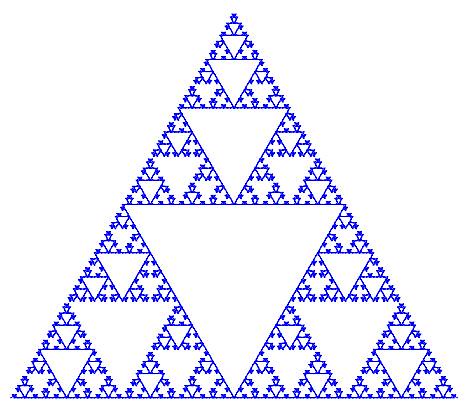
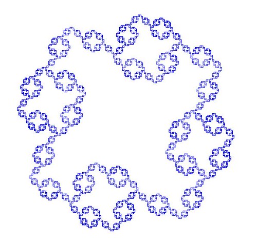
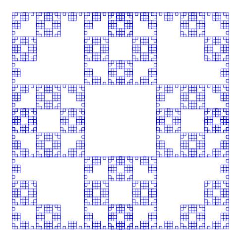
More on Lindenmayer Systems

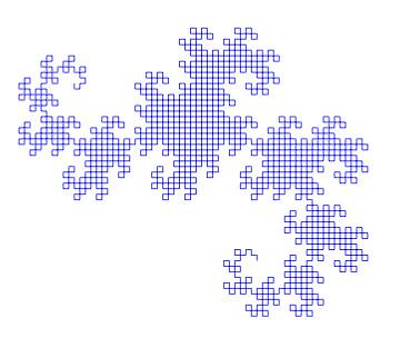
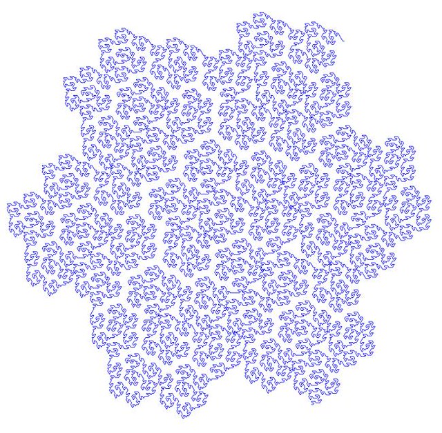
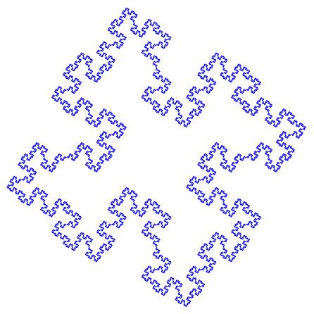
We briefly explored Lindenmayer systems (or L-systems) in an old post: Toying with Basic Fractals. We quickly reviewed this method for creation of an approximation to fractals, and displayed an example (the Koch snowflake) based on tikz libraries.

I would like to show a few more examples of beautiful curves generated with this technique, together with their generating axiom, rules and parameters. Feel free to click on each of the images below to download a larger version.

Note that any coding language with plotting capabilities should be able to tackle this project. I used once again tikz for , but this time with the tikzlibrary lindenmayersystems.

name : Dragon Curve axiom : X order : 11 step : 5pt angle : 90 rules : X -> X+YF+ Y -> -FX-Y	name : Gosper Space-filling Curve axiom : XF order : 5 step : 2pt angle : 60 rules : XF -> XF+YF++YF-XF--XFXF-YF+ YF -> -XF+YFYF++YF+XF--XF-YF
name : Quadric Koch Island axiom : F+F+F+F order : 4 step : 1pt angle : 90 rules : F -> F+F-F-FF+F+F-F	name : Sierpinski Arrowhead axiom : F order : 8 step : 3.5pt angle : 60 rules : G -> F+G+F F -> G-F-G
name : ? axiom : F+F+F+F order : 4 step : 2pt angle : 90 rules : F -> FF+F+F+F+F+F-F	name : ? axiom : F+F+F+F order : 4 step : 3pt angle : 90 rules : F -> FF+F+F+F+FF

Would you like to experiment a little with axioms, rules and parameters, and obtain some new pleasant curves with this method? If the mathematical properties of the fractal that they approximate are interesting enough, I bet you could attach your name to them. Like the astronomer that finds through her telescope a new object in the sky, or the zoologist that discover a new species of spider in the forest.

OpArt

OpArt is, by definition, a style of visual art based upon optical illusions. Let it be a painting, a photograph or any other mean, the objective of this style is to play with the interaction of what you see, and what it really is. A classical OpArt piece involves confusion by giving impression of movement, impossible solids, hidden images, conflicting patterns, warping, etc. And of course, Mathematics is a perfect vehicle to study—and even perform—this form of art.

In this post I would like to show an example of how to use trivial mathematics to implement a well-known example (shown above) in with the tikz package, and leave as homework another more interesting example.

Observe first the image above: the optical effect arises when conflicting concentric squares change the direction of their patterns. You may think that the color is the culprit of this effect but, as you will see below, it is only the relationship between the pure black-and-white patterns what produces the impression of movement.

Smallest Groups with Two Eyes

Today’s riddle is for the Go player. Your task is to find all the smallest groups with two eyes and place them all together (with the corresponding enclosing enemy stones) in a single board. Let me give you some tips first:

• Smallest groups in the corner: In the corner, six stones are the minimum needed to complete any group with two eyes. There are only four possibilities, and I took the liberty of placing them on the board for you:

  

• Smallest groups on the side: Consider any of the smallest groups with two eyes on a side of the board. How many stones do they have? [Hint: they all have the same number of stones] How many different groups are there?
• Smallest groups in the interior: Consider finally any of the smallest groups with two eyes in the interior of the board. How many stones do they have? [again, they all have the same number of stones]. How many different groups are there?

Since it is actually possible to place all those groups in the same board, this will help you figure out how many of each kind there are. Also, once finished, assume the board was obtained after a proper finished game (with no captures): What is the score?

Where are the powers of two?

The following construction gives an interesting pairing map between the positive integers and the lattice of integer-valued points in the plane:

• Place at the origin.
• For each level populate the points of the plane on the square with vertices starting from at the position and going counter-clockwise.

  

After pairing enough positive integers on the lattice, pay attention to the powers of two: they all seem to be located on the same two horizontal lines: and

Is this statement true?

The Cantor Pairing Function

The objective of this post is to construct a pairing function, that presents us with a bijection between the set of natural numbers, and the lattice of points in the plane with non-negative integer coordinates.

We will accomplish this by creating the corresponding map (and its inverse), that takes each natural number and drops it at a location in the lattice, as the following diagram suggests: