Edge detection: The Convolution Approach

Today I would like to show a very basic technique of detection based on simple convolution of an image with small kernels (masks). The purpose of these kernels is to enhance certain properties of the image at each pixel. What properties? Those that define what means to be an edge, in a differential calculus way—exactly as it was defined in the description of the Canny edge detector. The big idea is to assign to each pixel a numerical value that expresses its strength as an edge: positive if we suspect that such structure is present at that location, negative if not, and zero if the image is locally flat around that point. Masks can be designed so that they mimic the effect of differential operators, but these can be terribly complicated and give rise to large matrices.

The first approaches were performed with simple kernels. For example, Faler came up with the following four simple masks that emulate differentiation:

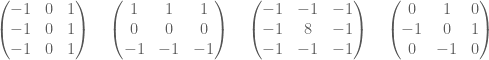
Note that, adding all the values of each matrix, one obtains zero. This is consistent with the third property required for our kernels: in the event of a locally flat area around a given pixel, convolution with any of these will offer a value of zero.

Read more…

Edge detection: The Scale Space Theory

Consider an image as a bounded function with no smoothness or structure assumptions a priori. Most relevant information of a given image is contained in the contours of the mapped objects: Think for example of a bright object against a dark background—the area where these two meet presents a curve where the intensity varies strongly. This is what we refer to as an “edge.”

Initially, we may consider the process of detection of an edge by the simple computation of the gradient This gradient should have a large intensity and a direction which indicates the perpendicular to the curve. It therefore looks sound to simply compute the gradient of and choose the points where these values are large. This conclusion is a bit unrealistic for two reasons:

1. The points where the gradient is larger than a given threshold are open sets, and thus don’t have the structure of curves.
2. Large gradient may arise in certain locations of the image due to tiny oscillations or noise, but completely unrelated to the objects being mapped. As a matter of fact, there is no reason to assume the existence or computability of any gradient at all in a given digital image.

Read more…

Image Processing with numpy, scipy and matplotlibs in sage

In this post, I would like to show how to use  a few different features of numpy, scipy and matplotlibs to accomplish a few basic image processing tasks: some trivial image manipulation, segmentation, obtaining of structural information, etc.  An excellent way to show a good set of these techniques is by working through a complex project.  In this case, I have chosen the following:

Given a HAADF-STEM micrograph of a bronze-type Niobium Tungsten oxide (left), find a script that constructs a good approximation to its structural model (right).

Courtesy of ETH Zurich

For pedagogical purposes, I took the following approach to solving this problem:

1. Segmentation of the atoms by thresholding and morphological operations.
2. Connected component labeling to extract each single atom for posterior examination.
3. Computation of the centers of mass of each label identified as an atom. This presents us with a lattice of points in the plane that shows a first insight in the structural model of the oxide.
4. Computation of Delaunay triangulation and Voronoi diagram of the previous lattice of points. The combination of information from these two graphs will lead us to a decent (approximation to the actual) structural model of our sample.

Let us proceed in this direction: